Linear Regression (Part 2)

3. Linear Regression (Part 2)#

3.1. Simple Linear Regression (Recap)#

A simple linear model relating a single feature, $x$, to an outcome $y$:

\[ y_i = \underbrace{\theta_0}_{\text{y intercept}} + \underbrace{\theta_1}_{\text{slope}} \cdot x_i + \epsilon_i \]

This is the equation of a line.

3.1.1. Fitting a linear model#

Goal $\theta_0$ and $\theta_1$ are our parameters; they are unknown. We want to find the values of $\theta_0$ and $\theta_1$ that best fit our data.

Goodness of Fit

Residual ($\epsilon_i$) - the difference between the actual target value $y_i$ and the model’s prediction $\hat{y}_i$, $\epsilon_i = y_i - \hat{y}_i$. We can think of a residual as an error.
Loss function - For any given data point, we penalize error using a loss function. The most common loss function is squared error, $\epsilon_i^2$.
Cost function - an aggregation of the loss over a set of data, usually the average of the individual losses. We assess the goodness-of-fit of a model using a cost function. The most common cost function is Mean Squared Error (MSE), the average of the squared error of all the data. The lower the cost, the better; lower cost means less error.
Best-fit model - the choice of $theta$’s that yield the lowest cost over the training or validation data set.

from sklearn.linear_model import LinearRegression
from sklearn.model_selection import train_test_split
from sklearn.datasets import make_regression
from sklearn.metrics import mean_squared_error

import numpy as np

import matplotlib.pyplot as plt

3.1.1.1. Creating synthetic data#

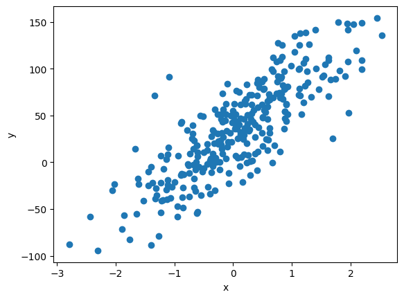
For a simple linear regression, we create a data set with just one feature and one target.

np.random.seed(1)
bias = 20*np.random.randn()

X, y, coef = make_regression(n_samples=300, 
                                   n_features=1,    # n_features = 1 --> simple linear regression
                                   noise=30, 
                                   bias = bias, 
                                   random_state=1, 
                                   shuffle = False, # samples will be in order
                                   coef = True) 

print(f'\'True\' model:\n y = {bias:.2f} + {coef:.2f} * x')


# plot the data
fig, ax = plt.subplots(1,1)
ax.scatter(X, y)
ax.set_xlabel('x')
ax.set_ylabel('y')
plt.show()

'True' model:
 y = 32.49 + 44.19 * x

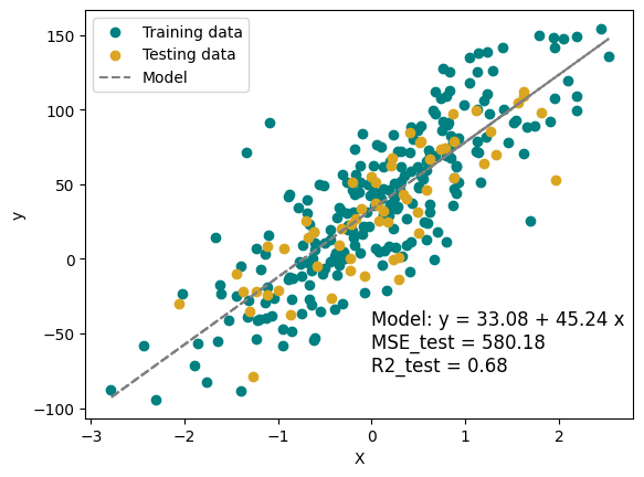
../_images/f0cfe1dd6af80b5fdae9201f4ba025feb65264558f3c47d67eaf135f85fc9c4b.png

3.1.1.2. Fitting the model#

In the cell block below, we do the following steps:

Split data into training and testing sets. Typically, we save 20% of the data for training.
Choose a model type and a choice of hyper-parameters. We choose LinearRegression as the model type, using the default hyper-parameters.
Fit the model and calculate MSE and $R^2$ for our training and testing sets.

# Split the data into training and testing sets, it's typical to save 20% of the data for testing
X_train, X_test, y_train, y_test = train_test_split(X, y, test_size=0.2, random_state=1)

# Create and train the model
model_LR = LinearRegression()
model_LR.fit(X_train, y_train)

# Make predictions
y_pred_train = model_LR.predict(X_train)
y_pred_test = model_LR.predict(X_test)
y_pred = model_LR.predict(X)

# Assess the model
MSE_train = mean_squared_error(y_train, y_pred_train)
R2_train = model_LR.score(X_train, y_train)

MSE_test = mean_squared_error(y_test, y_pred_test)
R2_test = model_LR.score(X_test, y_test)


print(f'model coefficients: {model_LR.coef_[0]}, {model_LR.intercept_}')
print(f'MSE_test = {MSE_test:.2f}, MSE_train = {MSE_train:.2f}')
print(f'R2_test = {R2_test:.2f}, R2_train = {R2_train:.2f}')

model_LR.__dict__

model coefficients: 45.24496021244698, 33.078033584023714
MSE_test = 580.18, MSE_train = 853.64
R2_test = 0.68, R2_train = 0.69

{'fit_intercept': True,
 'copy_X': True,
 'n_jobs': None,
 'positive': False,
 'n_features_in_': 1,
 'coef_': array([45.24496021]),
 'rank_': 1,
 'singular_': array([14.84030073]),
 'intercept_': np.float64(33.078033584023714)}

plt.scatter(X_train, y_train, color='teal', label='Training data')
plt.scatter(X_test, y_test, color='goldenrod', label='Testing data')
plt.plot(X, y_pred, color='gray', linestyle = '--', label='Model')

plt.xlabel('X')
plt.ylabel('y')
plt.text(0, -75, f'Model: y = {model_LR.intercept_:.2f} + {model_LR.coef_[0]:.2f} x \nMSE_test = {MSE_test:.2f}\nR2_test = {R2_test:.2f}', fontsize=12)

plt.legend()
plt.show()

../_images/7b1a51bcf3c44222e3c4bfef71068f1106de7ba7252f3a98992ea4ba1bc35102.png

3.1.2. Gradient Descent (A very brief aside)#

In the last class, we just tried a lot of different values for $\theta_0$ and $\theta_1$ (we tried about 1000 pairs) and picked the values that gave the lowest MSE. This is a brute force method and as our models get even slightly more complex, this method becomes impractical. So how does Scikit-learn fit models?

Recall that when we plot the MSE versus $\theta_0$ and $\theta_1$ we got a bowl shape. The minimum MSE (produced by the best model) is at the bottom of the bowl. Can we find the bottom of the bowl without knowing the entire bowl shape? Yes!

$\underbrace{\Theta_{new}}_{\text{our new guess}} = \underbrace{\Theta_{old}}_{\text{our old guess}} + \underbrace{\gamma}_{\text{learning rate}} \cdot \underbrace{\nabla J(\Theta)}_{\text{gradient of cost}}$

Gradient descent - an iterative algorithm for finding a (local) minimum of a function.

Start with a guess, any set of parameters $\theta$ for your model.
Calculate the gradient of the cost function at that point, say ($\theta_0$, $\theta_1$) for a simple linear regression. The gradient is the derivative (slope) of a function at a point. It is a vector, so it has a magnitude (how steep) and direction (where is it sloping).
Take a step downhill. The step size is determined by the gradient and learning rate.
Keep stepping until $\theta$ has converged, the change from step to step is small.

Comments

The learning rate contributes to step size.
- If learning rate is too low, you’ll take teeny tiny steps and your model might take a long time to fit.
- If learning rate is too high, you may step past your minimum.
The nice bowl shape is a convenience of linear regression. Not all regressions will have such a simple shape.
Some models will create cost landscapes with multiple minima. We want to find the global minimum (the lowest low), but gradient descent finds local minima. Solution, run gradient descent several times using different guesses or use a stochastic gradient descent method.

Okay that’s enough about that.

3.2. Multiple Linear Regression#

In Multiple Linear Regression, we predict the target $y$ using multiple features $x$.

$y = \theta_0 + \theta_1 \cdot x_1 + \theta_2 \cdot x_2 + \cdots + \theta_n \cdot x_n + \epsilon$

The process is very similar to simple linear regression. Let’s make some synthetic data with 2 features and 1 target.

For those with a background in linear algebra, the equation above can be represented in vector form as:

\[ y = \Theta^T X + \theta_0 + \epsilon \]

where:

$$ \Theta = \begin{bmatrix} \theta_1\ \theta_2\ \vdots \ \theta_n \end{bmatrix} \text{\qquad and \qquad} X = \begin{bmatrix} x_1\ x_2\ \vdots \ x_n \end{bmatrix}

np.random.seed(1)
bias = 20*np.random.randn()

X, y, coef = make_regression(n_samples=300, 
                                   n_features=2,    # n_features = 1 --> simple linear regression
                                   noise=30, 
                                   bias = bias, 
                                   random_state=1, 
                                   shuffle = False, # samples will be in order
                                   coef = True) 

print(f'\'True\' model:\n y = {bias:.2f} + {coef[0]:.2f} * x_1 + {coef[1]:.2f} * x_2')

# Uncomment the line below for an interactive figure
%matplotlib widget
from mpl_toolkits.mplot3d import Axes3D  

fig = plt.figure()
ax = fig.add_subplot(111, projection = '3d')

ax.scatter(X[:,0], X[:,1], y, s=5, alpha = 0.5)

ax.set_xlabel('x_1')
ax.set_ylabel('x_2')
ax.set_zlabel('y')

plt.show()

'True' model:
 y = 32.49 + 64.78 * x_1 + 17.98 * x_2

# Split the data into training and testing sets
X_train, X_test, y_train, y_test = train_test_split(X, y, test_size=0.2, random_state=1)

# Create and train the model
model_LR = LinearRegression()
model_LR.fit(X_train, y_train)

# Make predictions
y_pred_train = model_LR.predict(X_train)
y_pred_test = model_LR.predict(X_test)
y_pred = model_LR.predict(X)

# Assess the model
MSE_train = mean_squared_error(y_train, y_pred_train)
R2_train = model_LR.score(X_train, y_train)

MSE_test = mean_squared_error(y_test, y_pred_test)
R2_test = model_LR.score(X_test, y_test)


print(f'model coefficients: {model_LR.coef_}, {model_LR.intercept_}')
print(f'MSE_test = {MSE_test:.2f}, MSE_train = {MSE_train:.2f}')
print(f'R2_test = {R2_test:.2f}, R2_train = {R2_train:.2f}')

model_LR.__dict__

print(f'\nBest-fit Model:\n\ty = {model_LR.intercept_:.2f} + {model_LR.coef_[0]:.2f}*x_1 + {model_LR.coef_[1]:.2f}*x_2')

model coefficients: [63.82273891 20.71147598], 31.82452688535094
MSE_test = 747.16, MSE_train = 872.37
R2_test = 0.78, R2_train = 0.83

Best-fit Model:
	y = 31.82 + 63.82*x_1 + 20.71*x_2

np.random.seed(1)
bias = 20*np.random.randn()

X1, X2 = np.meshgrid(np.arange(-4,4,0.2), np.arange(-4,4,0.2))
X_grid = np.vstack((X1.flatten(), X2.flatten())).transpose()

y_pred_grid = model_LR.predict(X_grid)
y_pred_grid = y_pred_grid.reshape(X1.shape)

/Users/eatai/.pyenv/versions/3.13.1/envs/datascience/lib/python3.13/site-packages/sklearn/linear_model/_base.py:279: RuntimeWarning: divide by zero encountered in matmul
  return X @ coef_ + self.intercept_
/Users/eatai/.pyenv/versions/3.13.1/envs/datascience/lib/python3.13/site-packages/sklearn/linear_model/_base.py:279: RuntimeWarning: overflow encountered in matmul
  return X @ coef_ + self.intercept_
/Users/eatai/.pyenv/versions/3.13.1/envs/datascience/lib/python3.13/site-packages/sklearn/linear_model/_base.py:279: RuntimeWarning: invalid value encountered in matmul
  return X @ coef_ + self.intercept_

from mpl_toolkits.mplot3d import Axes3D  

fig = plt.figure()
ax = fig.add_subplot(111, projection = '3d')

ax.scatter(X[:,0], X[:,1], y, s=5, alpha = 0.5, label = 'Data')
ax.plot_surface(X1, X2, y_pred_grid, color = 'goldenrod', alpha = 0.5, label = 'Model')
ax.set_xlabel('x_1')
ax.set_ylabel('x_2')
ax.set_zlabel('y')

plt.show()

/Users/eatai/.pyenv/versions/3.13.1/envs/datascience/lib/python3.13/site-packages/mpl_toolkits/mplot3d/art3d.py:1403: RuntimeWarning: divide by zero encountered in matmul
  shade = ((normals / np.linalg.norm(normals, axis=1, keepdims=True))
/Users/eatai/.pyenv/versions/3.13.1/envs/datascience/lib/python3.13/site-packages/mpl_toolkits/mplot3d/art3d.py:1403: RuntimeWarning: overflow encountered in matmul
  shade = ((normals / np.linalg.norm(normals, axis=1, keepdims=True))

3.3. The modeling process#

Exploratory Data Analysis (today)
Clean data (today)
Engineer features (skip for now)
Pre-process data (skip for now)
Split data into training and testing sets. Possibly split training sets into training and validation sets.
Choose a model type and a choice of hyper-parameters.
Fit the model.
Assess the model.
If you’re unsatisfied with the results, go back as many steps as necessary and repeat.

3.3.1. Example: King County Housing#

In this example, we’ll be exploring how the attributes of a home (etc. size, condition, location, etc) contribute to its. Ultimately, we aim to predict sale price from the attributes.

For whom would this model be useful? How so?

3.3.1.1. Exploratory Data Analysis#

What questions might you ask to familiarize yourself with the data?

What are the columns? What do they represent? What are the units?
How big is the sample size?
Types of variables? (numeric, ints, floats)
Relationship the variables have with each other?
Missing data, data quality?
Plots (scatter, hist)
Describe, head, info.

import pandas as pd
import seaborn as sns

housing_df = pd.read_csv('https://raw.githubusercontent.com/GettysburgDataScience/datasets/refs/heads/main/kc_house_data.csv')

housing_df.info()

<class 'pandas.core.frame.DataFrame'>
RangeIndex: 21613 entries, 0 to 21612
Data columns (total 21 columns):
 #   Column         Non-Null Count  Dtype  
---  ------         --------------  -----  
 id             21613 non-null  int64  
 date           21613 non-null  object 
 price          21613 non-null  float64
 bedrooms       21613 non-null  int64  
 bathrooms      21613 non-null  float64
 sqft_living    21613 non-null  int64  
 sqft_lot       21613 non-null  int64  
 floors         21613 non-null  float64
 waterfront     21613 non-null  int64  
 view           21613 non-null  int64  
condition      21613 non-null  int64  
grade          21613 non-null  int64  
sqft_above     21613 non-null  int64  
sqft_basement  21613 non-null  int64  
yr_built       21613 non-null  int64  
yr_renovated   21613 non-null  int64  
zipcode        21613 non-null  int64  
lat            21613 non-null  float64
long           21613 non-null  float64
sqft_living15  21613 non-null  int64  
sqft_lot15     21613 non-null  int64  
dtypes: float64(5), int64(15), object(1)
memory usage: 3.5+ MB

housing_df.head(20)

	id	date	price	bedrooms	bathrooms	sqft_living	sqft_lot	floors	view	...	grade	sqft_above	sqft_basement	yr_built	yr_renovated	zipcode	lat	long	sqft_living15	sqft_lot15
0	7129300520	20141013T000000	221900.0	3	1.00	1180	5650	1.0	0	...	7	1180	0	1955	0	98178	47.5112	-122.257	1340	5650
1	6414100192	20141209T000000	538000.0	3	2.25	2570	7242	2.0	0	...	7	2170	400	1951	1991	98125	47.7210	-122.319	1690	7639
2	5631500400	20150225T000000	180000.0	2	1.00	770	10000	1.0	0	...	6	770	0	1933	0	98028	47.7379	-122.233	2720	8062
3	2487200875	20141209T000000	604000.0	4	3.00	1960	5000	1.0	0	...	7	1050	910	1965	0	98136	47.5208	-122.393	1360	5000
4	1954400510	20150218T000000	510000.0	3	2.00	1680	8080	1.0	0	...	8	1680	0	1987	0	98074	47.6168	-122.045	1800	7503
5	7237550310	20140512T000000	1225000.0	4	4.50	5420	101930	1.0	0	...	11	3890	1530	2001	0	98053	47.6561	-122.005	4760	101930
6	1321400060	20140627T000000	257500.0	3	2.25	1715	6819	2.0	0	...	7	1715	0	1995	0	98003	47.3097	-122.327	2238	6819
7	2008000270	20150115T000000	291850.0	3	1.50	1060	9711	1.0	0	...	7	1060	0	1963	0	98198	47.4095	-122.315	1650	9711
8	2414600126	20150415T000000	229500.0	3	1.00	1780	7470	1.0	0	...	7	1050	730	1960	0	98146	47.5123	-122.337	1780	8113
9	3793500160	20150312T000000	323000.0	3	2.50	1890	6560	2.0	0	...	7	1890	0	2003	0	98038	47.3684	-122.031	2390	7570
10	1736800520	20150403T000000	662500.0	3	2.50	3560	9796	1.0	0	...	8	1860	1700	1965	0	98007	47.6007	-122.145	2210	8925
11	9212900260	20140527T000000	468000.0	2	1.00	1160	6000	1.0	0	...	7	860	300	1942	0	98115	47.6900	-122.292	1330	6000
12	114101516	20140528T000000	310000.0	3	1.00	1430	19901	1.5	0	...	7	1430	0	1927	0	98028	47.7558	-122.229	1780	12697
13	6054650070	20141007T000000	400000.0	3	1.75	1370	9680	1.0	0	...	7	1370	0	1977	0	98074	47.6127	-122.045	1370	10208
14	1175000570	20150312T000000	530000.0	5	2.00	1810	4850	1.5	0	...	7	1810	0	1900	0	98107	47.6700	-122.394	1360	4850
15	9297300055	20150124T000000	650000.0	4	3.00	2950	5000	2.0	3	...	9	1980	970	1979	0	98126	47.5714	-122.375	2140	4000
16	1875500060	20140731T000000	395000.0	3	2.00	1890	14040	2.0	0	...	7	1890	0	1994	0	98019	47.7277	-121.962	1890	14018
17	6865200140	20140529T000000	485000.0	4	1.00	1600	4300	1.5	0	...	7	1600	0	1916	0	98103	47.6648	-122.343	1610	4300
18	16000397	20141205T000000	189000.0	2	1.00	1200	9850	1.0	0	...	7	1200	0	1921	0	98002	47.3089	-122.210	1060	5095
19	7983200060	20150424T000000	230000.0	3	1.00	1250	9774	1.0	0	...	7	1250	0	1969	0	98003	47.3343	-122.306	1280	8850

20 rows × 21 columns

housing_df.describe()

	id	price	bedrooms	bathrooms	sqft_living	sqft_lot	floors	waterfront	view	condition	grade	sqft_above	sqft_basement	yr_built	yr_renovated	zipcode	lat	long	sqft_living15	sqft_lot15
count	2.161300e+04	2.161300e+04	21613.000000	21613.000000	21613.000000	2.161300e+04	21613.000000	21613.000000	21613.000000	21613.000000	21613.000000	21613.000000	21613.000000	21613.000000	21613.000000	21613.000000	21613.000000	21613.000000	21613.000000	21613.000000
mean	4.580302e+09	5.400881e+05	3.370842	2.114757	2079.899736	1.510697e+04	1.494309	0.007542	0.234303	3.409430	7.656873	1788.390691	291.509045	1971.005136	84.402258	98077.939805	47.560053	-122.213896	1986.552492	12768.455652
std	2.876566e+09	3.671272e+05	0.930062	0.770163	918.440897	4.142051e+04	0.539989	0.086517	0.766318	0.650743	1.175459	828.090978	442.575043	29.373411	401.679240	53.505026	0.138564	0.140828	685.391304	27304.179631
min	1.000102e+06	7.500000e+04	0.000000	0.000000	290.000000	5.200000e+02	1.000000	0.000000	0.000000	1.000000	1.000000	290.000000	0.000000	1900.000000	0.000000	98001.000000	47.155900	-122.519000	399.000000	651.000000
25%	2.123049e+09	3.219500e+05	3.000000	1.750000	1427.000000	5.040000e+03	1.000000	0.000000	0.000000	3.000000	7.000000	1190.000000	0.000000	1951.000000	0.000000	98033.000000	47.471000	-122.328000	1490.000000	5100.000000
50%	3.904930e+09	4.500000e+05	3.000000	2.250000	1910.000000	7.618000e+03	1.500000	0.000000	0.000000	3.000000	7.000000	1560.000000	0.000000	1975.000000	0.000000	98065.000000	47.571800	-122.230000	1840.000000	7620.000000
75%	7.308900e+09	6.450000e+05	4.000000	2.500000	2550.000000	1.068800e+04	2.000000	0.000000	0.000000	4.000000	8.000000	2210.000000	560.000000	1997.000000	0.000000	98118.000000	47.678000	-122.125000	2360.000000	10083.000000
max	9.900000e+09	7.700000e+06	33.000000	8.000000	13540.000000	1.651359e+06	3.500000	1.000000	4.000000	5.000000	13.000000	9410.000000	4820.000000	2015.000000	2015.000000	98199.000000	47.777600	-121.315000	6210.000000	871200.000000

3.3.2. Selecting features#

When we have many features, we may want to select only a subset of features to use. How would we decide which features to use?

Correlation between two variables conveys the extent of a linear relationship between the two variables. The *correlation coefficient *, $\rho$, ranges from -1 to 1.

$\rho = 1$ is a perfect positive correlation. One variable is exactly linearly related to the other with positive slope.
$\rho = -1$ is a perfect negative correlation. One variable is exactly linearly related to the other with negative slope.
$\rho = 0$ suggests the two variables are completely uncorrelated.
$0 < |\rho| < 1$ suggests some correlation. The two variables might be linearly related, but not exactly due to noisy measurements, non-linearities, unconsidered factors, etc. What is considered good correlation varies from domain to domain.

We will want to select features that are correlated to the target value but not correlated to eachother (co-linearity). In the next section, we’ll see how to automate that selection.

Also…Correlation does not imply causation!:

Variables may be correlated to the same thing (e.g. ice cream purchases and heat stroke cases are both correlated to temperature).
Variables could be correlated by chance. See this site of Spurious Correlations

corr = housing_df.corr(numeric_only = True)

import seaborn as sns

fig, ax = plt.subplots(1, 1, figsize = (8, 8))
sns.heatmap(np.abs(corr), 
            vmin = 0, vmax = 1, 
            annot = True, 
            fmt = '.1f',
            ax = ax)
plt.show()

Maybe:

sqft living
view
lat

sns.pairplot(housing_df)
plt.show()