1. Classification

Classification tasks predict the categories, classes, or bins that data fall into. Classification tasks can be binary (e.g. deciding whether a product review was written by an actual customer or is AI-generated/paid review, identifying bank transactaions as legitimate or fraud, predicting how a registered voter will vote…assuming two political parties, etc.) or multi-class (e.g. what bird is making that call, what varietal of wine goes best with this meal, what major should a student pursue, etc).

We’ll start by focusing on binary classification tasks, introducing some concepts that apply to all such tasks. We’ll introduce some ways we assess classification models.

1.1. Binary classification

Binary classification assigns each data point (feature vector) to one of two categories, often referred to as Positive and Negative. It is important to define which of the two categories corresponds to Positive and which to Negative.

• Mushroom id: P = poisonous, N = edible

• Cancer classification: P = malignant, N = benign

• GenAI usage detector: P = AI generated, N = student written

Just as in regression, we’ll train our models on a training set and evaluate our models on the training and testing set. But instead of residuals, we have correct and incorrect identifications. For binary classification, correct predictions and mistakes are described as one of four groups:

Correct

• True Positive (TP) - a correct positive identification

• True Negative (TN) - a correct negative identification

Incorrect

• False Positive (FP) - a negative case that was mis-classified as positive

• False Negative (FN) - a positive case that was mis-classified as negative

In hypothesis testing, False Positives and False Negatives are often referred to as Type I and Type II errors respectively. Which is worse, FP or FN? Or is a mistake just a mistake?

It depends on the situation.

• Which is the more egregious errors for each of the examples above?

• Come up with two novel examples, one in which FP is the worse error and another in which FN is the worse error? Can you think of a general rule for which kind of error should be avoided?

1.1.1. An example

In the following example, we’ll use Logistic Regression (we’ll go into detail about this algorithm in the next lecture) to classify breast tumors as malignant or benign based on the physical properties of the tumor (e.g. size, shape, texture).

import matplotlib.pyplot as plt
import seaborn as sns

import numpy as np

from sklearn.datasets import load_breast_cancer
from sklearn.preprocessing  import StandardScaler
from sklearn.model_selection import train_test_split
from sklearn.linear_model import LogisticRegression
from sklearn.metrics import ConfusionMatrixDisplay

# Load the breast cancer dataset
bc_df, y = load_breast_cancer(return_X_y=True, as_frame=True)

# The original dataset maps 0=malignant, 1=benign. This feels backwards to me, so I swap 0 and 1
y = 1-y 
display(bc_df.describe())
display(y.describe())

	mean radius	mean texture	mean perimeter	mean area	mean smoothness	mean compactness	mean concavity	mean concave points	mean symmetry	mean fractal dimension	...	worst radius	worst texture	worst perimeter	worst area	worst smoothness	worst compactness	worst concavity	worst concave points	worst symmetry	worst fractal dimension
count	569.000000	569.000000	569.000000	569.000000	569.000000	569.000000	569.000000	569.000000	569.000000	569.000000	...	569.000000	569.000000	569.000000	569.000000	569.000000	569.000000	569.000000	569.000000	569.000000	569.000000
mean	14.127292	19.289649	91.969033	654.889104	0.096360	0.104341	0.088799	0.048919	0.181162	0.062798	...	16.269190	25.677223	107.261213	880.583128	0.132369	0.254265	0.272188	0.114606	0.290076	0.083946
std	3.524049	4.301036	24.298981	351.914129	0.014064	0.052813	0.079720	0.038803	0.027414	0.007060	...	4.833242	6.146258	33.602542	569.356993	0.022832	0.157336	0.208624	0.065732	0.061867	0.018061
min	6.981000	9.710000	43.790000	143.500000	0.052630	0.019380	0.000000	0.000000	0.106000	0.049960	...	7.930000	12.020000	50.410000	185.200000	0.071170	0.027290	0.000000	0.000000	0.156500	0.055040
25%	11.700000	16.170000	75.170000	420.300000	0.086370	0.064920	0.029560	0.020310	0.161900	0.057700	...	13.010000	21.080000	84.110000	515.300000	0.116600	0.147200	0.114500	0.064930	0.250400	0.071460
50%	13.370000	18.840000	86.240000	551.100000	0.095870	0.092630	0.061540	0.033500	0.179200	0.061540	...	14.970000	25.410000	97.660000	686.500000	0.131300	0.211900	0.226700	0.099930	0.282200	0.080040
75%	15.780000	21.800000	104.100000	782.700000	0.105300	0.130400	0.130700	0.074000	0.195700	0.066120	...	18.790000	29.720000	125.400000	1084.000000	0.146000	0.339100	0.382900	0.161400	0.317900	0.092080
max	28.110000	39.280000	188.500000	2501.000000	0.163400	0.345400	0.426800	0.201200	0.304000	0.097440	...	36.040000	49.540000	251.200000	4254.000000	0.222600	1.058000	1.252000	0.291000	0.663800	0.207500

8 rows × 30 columns

count    569.000000
mean       0.372583
std        0.483918
min        0.000000
25%        0.000000
50%        0.000000
75%        1.000000
max        1.000000
Name: target, dtype: float64

%%capture
# Split the dataset into training and testing sets
X_train, X_test, y_train, y_test = train_test_split(bc_df, y, test_size=0.2, random_state=42)

# Standardize the features
scaler = StandardScaler()
X_train_scaled = scaler.fit_transform(X_train)
X_test_scaled = scaler.transform(X_test)

# Train a logistic regression model
model = LogisticRegression()
model.fit(X_train_scaled, y_train)

# Make predictions
y_pred = model.predict(X_test_scaled)
y_prob = model.predict_proba(X_test_scaled)

model.__dict__

{'penalty': 'l2',
 'dual': False,
 'tol': 0.0001,
 'C': 1.0,
 'fit_intercept': True,
 'intercept_scaling': 1,
 'class_weight': None,
 'random_state': None,
 'solver': 'lbfgs',
 'max_iter': 100,
 'multi_class': 'deprecated',
 'verbose': 0,
 'warm_start': False,
 'n_jobs': None,
 'l1_ratio': None,
 'n_features_in_': 30,
 'classes_': array([0, 1]),
 'n_iter_': array([20], dtype=int32),
 'coef_': array([[ 0.43190368,  0.38732553,  0.39343248,  0.46521006,  0.07166728,
         -0.54016395,  0.8014581 ,  1.11980408, -0.23611852, -0.07592093,
          1.26817815, -0.18887738,  0.61058302,  0.9071857 ,  0.31330675,
         -0.68249145, -0.17527452,  0.3112999 , -0.50042502, -0.61622993,
          0.87984024,  1.35060559,  0.58945273,  0.84184594,  0.54416967,
         -0.01611019,  0.94305313,  0.77821726,  1.20820031,  0.15741387]]),
 'intercept_': array([-0.44558453])}

coefs = model.coef_.flatten()
feature_names = np.array(bc_df.columns)

idx = np.argsort(np.abs(coefs))[::-1]

coefs = coefs[idx]
feature_names = feature_names[idx]

for f,c in zip(feature_names, coefs):
    print(f'{c:6.3f}\t{f}')

 1.351	worst texture
 1.268	radius error
 1.208	worst symmetry
 1.120	mean concave points
 0.943	worst concavity
 0.907	area error
 0.880	worst radius
 0.842	worst area
 0.801	mean concavity
 0.778	worst concave points
-0.682	compactness error
-0.616	fractal dimension error
 0.611	perimeter error
 0.589	worst perimeter
 0.544	worst smoothness
-0.540	mean compactness
-0.500	symmetry error
 0.465	mean area
 0.432	mean radius
 0.393	mean perimeter
 0.387	mean texture
 0.313	smoothness error
 0.311	concave points error
-0.236	mean symmetry
-0.189	texture error
-0.175	concavity error
 0.157	worst fractal dimension
-0.076	mean fractal dimension
 0.072	mean smoothness
-0.016	worst compactness

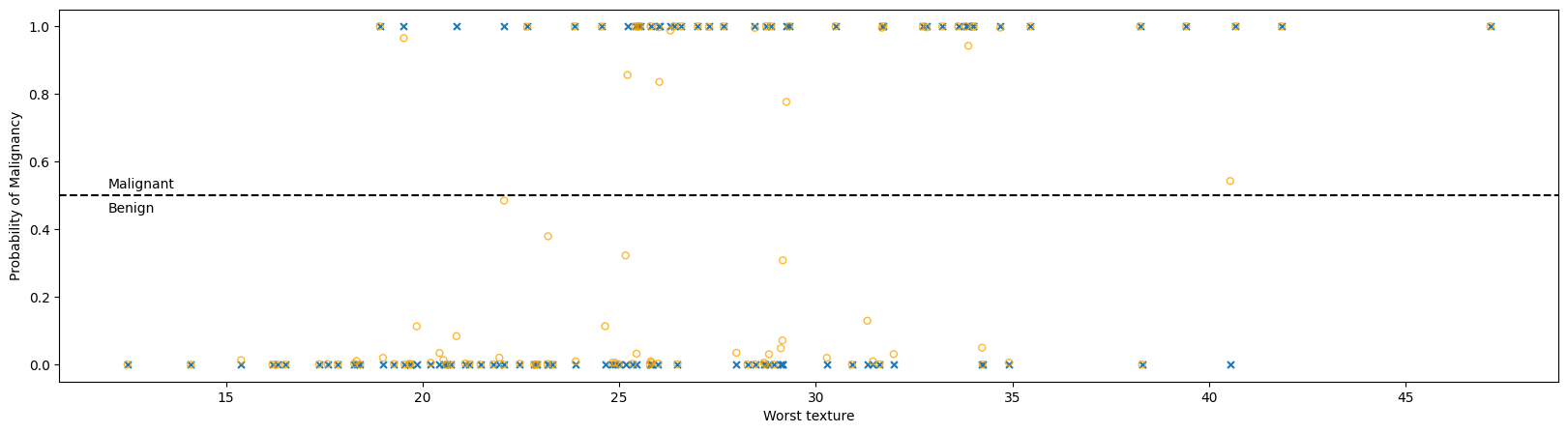
plt.subplots(1,1, figsize = (20, 5))
plt.scatter(X_test['worst texture'], y_test, label = 'True',
            s = 25, marker = 'x')

plt.scatter(X_test['worst texture'], y_prob[:,1], label = 'Predicted Probability', 
            s = 25, 
            alpha = 0.8, marker = 'o', ec = 'orange', facecolor = 'none')

# plt.scatter(X_test['worst texture'], y_pred, label = 'Predicted', 
#             s = 25, 
#             alpha = 0.8, marker = 'o', ec = 'r', facecolor = 'none')

plt.axhline(0.5, c = 'k', ls = '--')
plt.text(12, 0.52, 'Malignant')
plt.text(12, 0.45, 'Benign')

plt.xlabel('Worst texture')
plt.ylabel('Probability of Malignancy')
plt.show()

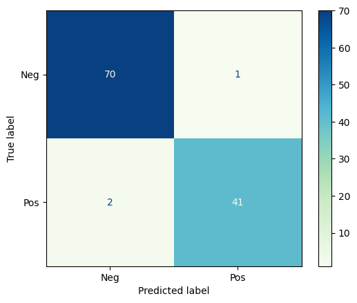
1.1.2. Confusion Matrix

The Confusion Matrix is a graphical representation of the predictions a classifier has made on the data set. The confusion matrix is an nxn grid where n is the number of categories; for binary classification, the confusion matrix is always 2x2.

Let’s look at the confusion matrix for the breast tumor classification above.

ConfusionMatrixDisplay.from_predictions(y_test, y_pred, 
                                        # normalize = 'true',
                                        # display_labels = ['Benign', 'Malignant'],
                                        display_labels = ['Neg', 'Pos'],
                                        cmap = 'GnBu'
                                        )
plt.show()

1.1.3. Binary classification metrics

There are also several metrics commonly used in binary classification: Accuracy, Precision, Recall, F1 score

• Accuracy - The percentage of correct predictions overall

  \[ \text{Accuracy} = \frac{TP + TN}{TP+TN+FP+FN} \]

• Precision - The percentage of positive predictions that were correct

  \[ \text{Precision} = \frac{TP}{TP + FP} \]

• Recall - The percentage of positive cases predicted correctly

  \[ \text{Recall} = \frac{TP}{TP+FN} \]

• F1 score - A hybrid metric comprising precision and recall

  \[ \text{F1} = \frac{2 \cdot Precision \cdot Recall}{Precision + Recall} = \frac{2 \cdot TP}{2 \cdot TP + FP + FN} \]

Now you try

Calculate the accuracy, precision, recall, and F1 score (by hand) for the confusion matrix above. Which metric is most useful/appropriate for this classification problem.

from sklearn.metrics import classification_report, PrecisionRecallDisplay

cr = classification_report(y_test, y_pred, target_names = ['Benign', 'Malignant'])
print(cr)

              precision    recall  f1-score   support

      Benign       0.97      0.99      0.98        71
   Malignant       0.98      0.95      0.96        43

    accuracy                           0.97       114
   macro avg       0.97      0.97      0.97       114
weighted avg       0.97      0.97      0.97       114

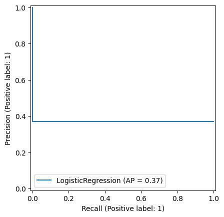
PrecisionRecallDisplay.from_estimator(model, X_train, y_train)
plt.show()

/Users/eatai/.pyenv/versions/3.13.1/envs/datascience/lib/python3.13/site-packages/sklearn/utils/validation.py:2732: UserWarning: X has feature names, but LogisticRegression was fitted without feature names
  warnings.warn(
/Users/eatai/.pyenv/versions/3.13.1/envs/datascience/lib/python3.13/site-packages/sklearn/utils/extmath.py:203: RuntimeWarning: divide by zero encountered in matmul
  ret = a @ b
/Users/eatai/.pyenv/versions/3.13.1/envs/datascience/lib/python3.13/site-packages/sklearn/utils/extmath.py:203: RuntimeWarning: overflow encountered in matmul
  ret = a @ b
/Users/eatai/.pyenv/versions/3.13.1/envs/datascience/lib/python3.13/site-packages/sklearn/utils/extmath.py:203: RuntimeWarning: invalid value encountered in matmul
  ret = a @ b