6. Forests and Trees#
Ensemble methods combine predictions across multiple models to improve prediction.
weak learners - simple models that predict slightly better than random guessing
strong learners - more complex models that predict significantly better than chance
6.1. Random Forests (RandomForestClassifier)#
A random forest creates numerous trees in parallel (at the same time). Each tree is relatively shallow, sometimes only a single node (called a stump).
To make a prediction, a sample is processed by each tree, each tree makes a prediction, and the majority vote wins. But what makes the trees in the forest different from each other?
In fitting, diversity of trees is created using two methods: feature selection and bagging.
6.1.1. Random feature subsets#
Each tree only gets a subset of the features. For example, in a random forest deciding whether or not you should buy a car, one tree might make a prediction based on [‘reliability’, ‘feul economy’, ‘price’], while another uses [‘top speed’, ‘interior room’, ‘cost to repair’], and another uses [‘resale value’, ‘feul economy’, ‘value of standard tech’] and another…
6.1.2. Bagging (Bootstrap aggregating)#
Bootstrapping is a method for creating new data sets by sampling existing data sets. In bootstrapping, you select samples randomly and allow a sample to be selected multiple times (called sampling with replacement).
Bagging is a method that uses bootstrapping to create different training sets for each tree, and then aggregating the results.
6.1.3. Why it works?#
The idea is that no one tree will be great, but they’ll all make different mistakes. But there’ll be more overlap in correct guesses than in mistakes. So for any given sample, the majority vote is more likely to be correct than any one tree.
6.2. Gradient Boosted Trees#
Whereas Random Forests fit trees in parallel and every tree gets an equal vote, Boosted trees create trees sequentially, each new tree focusing on the shortcomings of the previous. And at the voting stage, some trees get more say than others.
There are many flavors of Boosted trees: AdaBoost, XGBoost, CatBoost
They all work a little differently, but here’s an outline of AdaBoost as an example:
6.2.1. AdaBoost (Adaptive Boosting) ( GradientBoostingClassifier)#
In AdaBoost, a tree comprises only one decision node; this kind of tree is called a stump. In each iteration, a new stump is created that splits the data based on a different condition. As the algorithm iterates, it keeps track of:
Sample Weight - each iteration, the algorithm focuses more on misclassified samples.
A sample that is classified correctly is down-weighted. We get this right, don’t spend more energy on this case.
A sample that is classified incorrectly is up-weighted. We get this wrong, focus on this case.
Tree Influence - how much say a tree will have in the final vote. Trees that do better at classifying get more say.
A tree that is 50% correct gets no say. This tree is just guessing
A tree that is >50% gets a positive vote (0 to infinity). A tree that is 100% correct gets infinite vote! Listen to that tree!
A tree that is <50% gets a negative vote (0 to -infinity). A tree that is 0% correct gets a -infinite vote! Do the opposite of that tree!
The AdaBoost process:
Start with all the samples each counts the same.
Same as in a decision tree, pick a question that splits the data to minimize Gini Impurity.
Sum up sample weights for mis-classified samples and calculate Tree Influence.
Assign new weights to samples, increasing weights on mistakes and decreasing weights on correct classifications.
Create new stump, and repeat 2-5 until classification error is below some threshold you choose.
When you predict, you feed the sample through all the stumps and each votes according to their influence.
6.2.2. Example: Spam email prediction#
# !pip install ucimlrepo
from ucimlrepo import fetch_ucirepo
import pandas as pd

# fetch dataset
spambase = fetch_ucirepo(id=94)

# data (as pandas dataframes)
X = spambase.data.features
Y = spambase.data.targets

# to make y a compatible shape for sklearn models
y = Y['Class']
labels = ['ham', 'spam']

# metadata
print(spambase.metadata)

# variable information
print(spambase.variables)
{'uci_id': 94, 'name': 'Spambase', 'repository_url': 'https://archive.ics.uci.edu/dataset/94/spambase', 'data_url': 'https://archive.ics.uci.edu/static/public/94/data.csv', 'abstract': 'Classifying Email as Spam or Non-Spam', 'area': 'Computer Science', 'tasks': ['Classification'], 'characteristics': ['Multivariate'], 'num_instances': 4601, 'num_features': 57, 'feature_types': ['Integer', 'Real'], 'demographics': [], 'target_col': ['Class'], 'index_col': None, 'has_missing_values': 'no', 'missing_values_symbol': None, 'year_of_dataset_creation': 1999, 'last_updated': 'Mon Aug 28 2023', 'dataset_doi': '10.24432/C53G6X', 'creators': ['Mark Hopkins', 'Erik Reeber', 'George Forman', 'Jaap Suermondt'], 'intro_paper': None, 'additional_info': {'summary': 'The "spam" concept is diverse: advertisements for products/web sites, make money fast schemes, chain letters, pornography...\n\nThe classification task for this dataset is to determine whether a given email is spam or not.\n\t\nOur collection of spam e-mails came from our postmaster and individuals who had filed spam.  Our collection of non-spam e-mails came from filed work and personal e-mails, and hence the word \'george\' and the area code \'650\' are indicators of non-spam.  These are useful when constructing a personalized spam filter.  One would either have to blind such non-spam indicators or get a very wide collection of non-spam to generate a general purpose spam filter.\n\nFor background on spam: Cranor, Lorrie F., LaMacchia, Brian A.  Spam!, Communications of the ACM, 41(8):74-83, 1998.\n\nTypical performance is around ~7% misclassification error. False positives (marking good mail as spam) are very undesirable.If we insist on zero false positives in the training/testing set, 20-25% of the spam passed through the filter. See also Hewlett-Packard Internal-only Technical Report. External version forthcoming. ', 'purpose': None, 'funded_by': None, 'instances_represent': 'Emails', 'recommended_data_splits': None, 'sensitive_data': None, 'preprocessing_description': None, 'variable_info': 'The last column of \'spambase.data\' denotes whether the e-mail was considered spam (1) or not (0), i.e. unsolicited commercial e-mail.  Most of the attributes indicate whether a particular word or character was frequently occuring in the e-mail.  The run-length attributes (55-57) measure the length of sequences of consecutive capital letters.  For the statistical measures of each attribute, see the end of this file.  Here are the definitions of the attributes:\r\n\r\n48 continuous real [0,100] attributes of type word_freq_WORD \r\n= percentage of words in the e-mail that match WORD, i.e. 100 * (number of times the WORD appears in the e-mail) / total number of words in e-mail.  A "word" in this case is any string of alphanumeric characters bounded by non-alphanumeric characters or end-of-string.\r\n\r\n6 continuous real [0,100] attributes of type char_freq_CHAR] \r\n= percentage of characters in the e-mail that match CHAR, i.e. 100 * (number of CHAR occurences) / total characters in e-mail\r\n\r\n1 continuous real [1,...] attribute of type capital_run_length_average \r\n= average length of uninterrupted sequences of capital letters\r\n\r\n1 continuous integer [1,...] attribute of type capital_run_length_longest \r\n= length of longest uninterrupted sequence of capital letters\r\n\r\n1 continuous integer [1,...] attribute of type capital_run_length_total \r\n= sum of length of uninterrupted sequences of capital letters \r\n= total number of capital letters in the e-mail\r\n\r\n1 nominal {0,1} class attribute of type spam\r\n= denotes whether the e-mail was considered spam (1) or not (0), i.e. unsolicited commercial e-mail.  \r\n', 'citation': None}}
                          name     role        type demographic  \
0               word_freq_make  Feature  Continuous        None
1            word_freq_address  Feature  Continuous        None
2                word_freq_all  Feature  Continuous        None
3                 word_freq_3d  Feature  Continuous        None
4                word_freq_our  Feature  Continuous        None
5               word_freq_over  Feature  Continuous        None
6             word_freq_remove  Feature  Continuous        None
7           word_freq_internet  Feature  Continuous        None
8              word_freq_order  Feature  Continuous        None
9               word_freq_mail  Feature  Continuous        None
10           word_freq_receive  Feature  Continuous        None
11              word_freq_will  Feature  Continuous        None
12            word_freq_people  Feature  Continuous        None
13            word_freq_report  Feature  Continuous        None
14         word_freq_addresses  Feature  Continuous        None
15              word_freq_free  Feature  Continuous        None
16          word_freq_business  Feature  Continuous        None
17             word_freq_email  Feature  Continuous        None
18               word_freq_you  Feature  Continuous        None
19            word_freq_credit  Feature  Continuous        None
20              word_freq_your  Feature  Continuous        None
21              word_freq_font  Feature  Continuous        None
22               word_freq_000  Feature  Continuous        None
23             word_freq_money  Feature  Continuous        None
24                word_freq_hp  Feature  Continuous        None
25               word_freq_hpl  Feature  Continuous        None
26            word_freq_george  Feature  Continuous        None
27               word_freq_650  Feature  Continuous        None
28               word_freq_lab  Feature  Continuous        None
29              word_freq_labs  Feature  Continuous        None
30            word_freq_telnet  Feature  Continuous        None
31               word_freq_857  Feature  Continuous        None
32              word_freq_data  Feature  Continuous        None
33               word_freq_415  Feature  Continuous        None
34                word_freq_85  Feature  Continuous        None
35        word_freq_technology  Feature  Continuous        None
36              word_freq_1999  Feature  Continuous        None
37             word_freq_parts  Feature  Continuous        None
38                word_freq_pm  Feature  Continuous        None
39            word_freq_direct  Feature  Continuous        None
40                word_freq_cs  Feature  Continuous        None
41           word_freq_meeting  Feature  Continuous        None
42          word_freq_original  Feature  Continuous        None
43           word_freq_project  Feature  Continuous        None
44                word_freq_re  Feature  Continuous        None
45               word_freq_edu  Feature  Continuous        None
46             word_freq_table  Feature  Continuous        None
47        word_freq_conference  Feature  Continuous        None
48                 char_freq_;  Feature  Continuous        None
49                 char_freq_(  Feature  Continuous        None
50                 char_freq_[  Feature  Continuous        None
51                 char_freq_!  Feature  Continuous        None
52                 char_freq_$  Feature  Continuous        None
53                 char_freq_#  Feature  Continuous        None
54  capital_run_length_average  Feature  Continuous        None
55  capital_run_length_longest  Feature  Continuous        None
56    capital_run_length_total  Feature  Continuous        None
57                       Class   Target      Binary        None

                 description units missing_values
0                       None  None             no
1                       None  None             no
2                       None  None             no
3                       None  None             no
4                       None  None             no
5                       None  None             no
6                       None  None             no
7                       None  None             no
8                       None  None             no
9                       None  None             no
10                      None  None             no
11                      None  None             no
12                      None  None             no
13                      None  None             no
14                      None  None             no
15                      None  None             no
16                      None  None             no
17                      None  None             no
18                      None  None             no
19                      None  None             no
20                      None  None             no
21                      None  None             no
22                      None  None             no
23                      None  None             no
24                      None  None             no
25                      None  None             no
26                      None  None             no
27                      None  None             no
28                      None  None             no
29                      None  None             no
30                      None  None             no
31                      None  None             no
32                      None  None             no
33                      None  None             no
34                      None  None             no
35                      None  None             no
36                      None  None             no
37                      None  None             no
38                      None  None             no
39                      None  None             no
40                      None  None             no
41                      None  None             no
42                      None  None             no
43                      None  None             no
44                      None  None             no
45                      None  None             no
46                      None  None             no
47                      None  None             no
48                      None  None             no
49                      None  None             no
50                      None  None             no
51                      None  None             no
52                      None  None             no
53                      None  None             no
54                      None  None             no
55                      None  None             no
56                      None  None             no
57  spam (1) or not spam (0)  None             no
X.describe()
| word_freq_make | word_freq_address | word_freq_all | word_freq_3d | word_freq_our | word_freq_over | word_freq_remove | word_freq_internet | word_freq_order | word_freq_mail | ... | word_freq_conference | char_freq_; | char_freq_( | char_freq_[ | char_freq_! | char_freq_$ | char_freq_# | capital_run_length_average | capital_run_length_longest | capital_run_length_total | |
|---|---|---|---|---|---|---|---|---|---|---|---|---|---|---|---|---|---|---|---|---|---|
| count | 4601.000000 | 4601.000000 | 4601.000000 | 4601.000000 | 4601.000000 | 4601.000000 | 4601.000000 | 4601.000000 | 4601.000000 | 4601.000000 | ... | 4601.000000 | 4601.000000 | 4601.000000 | 4601.000000 | 4601.000000 | 4601.000000 | 4601.000000 | 4601.000000 | 4601.000000 | 4601.000000 |
| mean | 0.104553 | 0.213015 | 0.280656 | 0.065425 | 0.312223 | 0.095901 | 0.114208 | 0.105295 | 0.090067 | 0.239413 | ... | 0.031869 | 0.038575 | 0.139030 | 0.016976 | 0.269071 | 0.075811 | 0.044238 | 5.191515 | 52.172789 | 283.289285 |
| std | 0.305358 | 1.290575 | 0.504143 | 1.395151 | 0.672513 | 0.273824 | 0.391441 | 0.401071 | 0.278616 | 0.644755 | ... | 0.285735 | 0.243471 | 0.270355 | 0.109394 | 0.815672 | 0.245882 | 0.429342 | 31.729449 | 194.891310 | 606.347851 |
| min | 0.000000 | 0.000000 | 0.000000 | 0.000000 | 0.000000 | 0.000000 | 0.000000 | 0.000000 | 0.000000 | 0.000000 | ... | 0.000000 | 0.000000 | 0.000000 | 0.000000 | 0.000000 | 0.000000 | 0.000000 | 1.000000 | 1.000000 | 1.000000 |
| 25% | 0.000000 | 0.000000 | 0.000000 | 0.000000 | 0.000000 | 0.000000 | 0.000000 | 0.000000 | 0.000000 | 0.000000 | ... | 0.000000 | 0.000000 | 0.000000 | 0.000000 | 0.000000 | 0.000000 | 0.000000 | 1.588000 | 6.000000 | 35.000000 |
| 50% | 0.000000 | 0.000000 | 0.000000 | 0.000000 | 0.000000 | 0.000000 | 0.000000 | 0.000000 | 0.000000 | 0.000000 | ... | 0.000000 | 0.000000 | 0.065000 | 0.000000 | 0.000000 | 0.000000 | 0.000000 | 2.276000 | 15.000000 | 95.000000 |
| 75% | 0.000000 | 0.000000 | 0.420000 | 0.000000 | 0.380000 | 0.000000 | 0.000000 | 0.000000 | 0.000000 | 0.160000 | ... | 0.000000 | 0.000000 | 0.188000 | 0.000000 | 0.315000 | 0.052000 | 0.000000 | 3.706000 | 43.000000 | 266.000000 |
| max | 4.540000 | 14.280000 | 5.100000 | 42.810000 | 10.000000 | 5.880000 | 7.270000 | 11.110000 | 5.260000 | 18.180000 | ... | 10.000000 | 4.385000 | 9.752000 | 4.081000 | 32.478000 | 6.003000 | 19.829000 | 1102.500000 | 9989.000000 | 15841.000000 |
8 rows × 57 columns
6.2.3. Example: Palmer Penguins#
# palmer = pd.read_csv('https://gist.githubusercontent.com/slopp/ce3b90b9168f2f921784de84fa445651/raw/4ecf3041f0ed4913e7c230758733948bc561f434/penguins.csv', index_col = 'rowid')

# palmer.dropna(axis = 0, inplace=True)
# palmer.reset_index(drop = True, inplace=True)

# features = ['bill_length_mm', 'bill_depth_mm',
#        'flipper_length_mm', 'body_mass_g']

# target = 'species'
# labels = ['Adelie', 'Chinstrap', 'Gentoo']

# X = palmer[features]
# y = palmer[target]
from sklearn.tree import DecisionTreeClassifier
from sklearn.ensemble import RandomForestClassifier, GradientBoostingClassifier
from sklearn.model_selection import GridSearchCV, train_test_split


# Split data
X_train, X_test, y_train, y_test = train_test_split(X, y, test_size=0.5, random_state=42)

# Decision Tree
dt_params = {'max_depth': [3, 6, 9, None], 'min_samples_split': [2, 5, 10]}
dt_grid = GridSearchCV(DecisionTreeClassifier(random_state=42), dt_params, cv=5, n_jobs=-1)
dt_grid.fit(X_train, y_train)

# Random Forest
rf_params = {'n_estimators': [10, 30, 100], 'max_depth': [1, 2]}
rf_grid = GridSearchCV(RandomForestClassifier(random_state=42), rf_params, cv=5, n_jobs=-1)
rf_grid.fit(X_train, y_train)

# Gradient Boosted Trees
gb_params = {'n_estimators': [10, 30, 100], 'max_depth': [1, 2]}
gb_grid = GridSearchCV(GradientBoostingClassifier(random_state=42), gb_params, cv=5, n_jobs=-1)
gb_grid.fit(X_train, y_train)


# Get the best models
print("Best Decision Tree params:", dt_grid.best_params_)
print("Best Random Forest params:", rf_grid.best_params_)
print("Best Gradient Boosted params:", gb_grid.best_params_)

tree = dt_grid.best_estimator_
forest = rf_grid.best_estimator_
boosted = gb_grid.best_estimator_
Best Decision Tree params: {'max_depth': 6, 'min_samples_split': 10}
Best Random Forest params: {'max_depth': 2, 'n_estimators': 100}
Best Gradient Boosted params: {'max_depth': 2, 'n_estimators': 100}
y_tree_train = tree.predict(X_train)
y_tree_test = tree.predict(X_test)

y_forest_train = forest.predict(X_train)
y_forest_test = forest.predict(X_test)

y_boosted_train = boosted.predict(X_train)
y_boosted_test = boosted.predict(X_test)
from sklearn.metrics import confusion_matrix, ConfusionMatrixDisplay, classification_report
import matplotlib.pyplot as plt
models = [
('Decision Tree', y_tree_train, y_tree_test),
('Random Forest', y_forest_train, y_forest_test),
('Gradient Boosted', y_boosted_train, y_boosted_test)
]
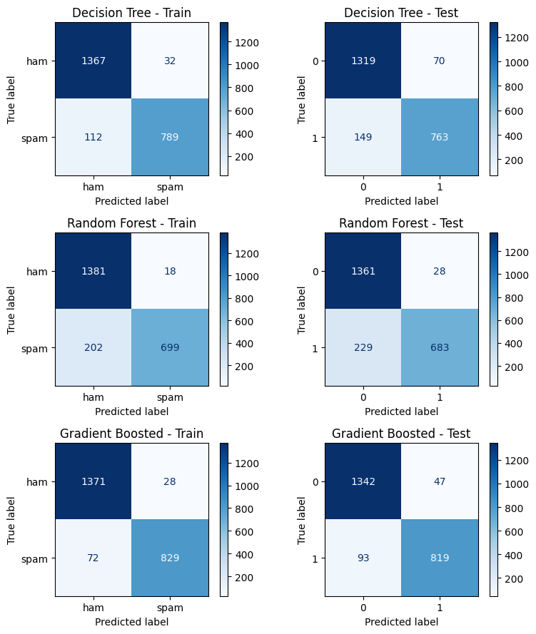
fig, axes = plt.subplots(3, 2, figsize=(8, 9))
for i, (name, y_pred_train, y_pred_test) in enumerate(models):
cm_train = confusion_matrix(y_train, y_pred_train)
cm_test = confusion_matrix(y_test, y_pred_test)
disp_train = ConfusionMatrixDisplay(cm_train, display_labels=labels)
disp_test = ConfusionMatrixDisplay(cm_test)
disp_train.plot(ax=axes[i, 0], cmap='Blues', values_format='d')
axes[i, 0].set_title(f'{name} - Train')
disp_test.plot(ax=axes[i, 1], cmap='Blues', values_format='d')
axes[i, 1].set_title(f'{name} - Test')
plt.tight_layout()
import numpy as np

def display_feature_importance(model):
    imps = model.feature_importances_
    features = model.feature_names_in_

    sort_idx = np.argsort(imps)[::-1]
    imps = imps[sort_idx]
    features = features[sort_idx]

    for k, (feature, imp) in enumerate(zip(features, imps), start = 1):
        print(f'{k:>3}. {feature:_<30}{imp:.4f}')
print('\nDECISION TREE\n====================================')
display_feature_importance(tree)
DECISION TREE
====================================
  1. char_freq_$___________________0.4501
  2. word_freq_remove______________0.2068
  3. char_freq_!___________________0.0992
  4. word_freq_hp__________________0.0598
  5. capital_run_length_total______0.0470
  6. word_freq_free________________0.0320
  7. word_freq_edu_________________0.0168
  8. word_freq_george______________0.0163
  9. word_freq_000_________________0.0162
 10. capital_run_length_longest____0.0110
 11. word_freq_you_________________0.0108
 12. capital_run_length_average____0.0089
 13. word_freq_1999________________0.0081
 14. word_freq_hpl_________________0.0066
 15. word_freq_email_______________0.0038
 16. word_freq_over________________0.0023
 17. word_freq_conference__________0.0022
 18. word_freq_mail________________0.0022
 19. word_freq_font________________0.0000
 20. word_freq_business____________0.0000
 21. word_freq_your________________0.0000
 22. word_freq_credit______________0.0000
 23. word_freq_address_____________0.0000
 24. word_freq_report______________0.0000
 25. word_freq_addresses___________0.0000
 26. word_freq_all_________________0.0000
 27. word_freq_people______________0.0000
 28. word_freq_will________________0.0000
 29. word_freq_order_______________0.0000
 30. word_freq_internet____________0.0000
 31. word_freq_our_________________0.0000
 32. word_freq_3d__________________0.0000
 33. word_freq_receive_____________0.0000
 34. word_freq_lab_________________0.0000
 35. word_freq_money_______________0.0000
 36. word_freq_cs__________________0.0000
 37. char_freq_#___________________0.0000
 38. char_freq_[___________________0.0000
 39. char_freq_(___________________0.0000
 40. char_freq_;___________________0.0000
 41. word_freq_table_______________0.0000
 42. word_freq_re__________________0.0000
 43. word_freq_project_____________0.0000
 44. word_freq_original____________0.0000
 45. word_freq_meeting_____________0.0000
 46. word_freq_direct______________0.0000
 47. word_freq_650_________________0.0000
 48. word_freq_pm__________________0.0000
 49. word_freq_parts_______________0.0000
 50. word_freq_technology__________0.0000
 51. word_freq_85__________________0.0000
 52. word_freq_415_________________0.0000
 53. word_freq_data________________0.0000
 54. word_freq_857_________________0.0000
 55. word_freq_telnet______________0.0000
 56. word_freq_labs________________0.0000
 57. word_freq_make________________0.0000
print('\nRANDOM FOREST\n====================================')
display_feature_importance(forest)
RANDOM FOREST
====================================
  1. char_freq_$___________________0.1412
  2. char_freq_!___________________0.1224
  3. word_freq_remove______________0.1150
  4. word_freq_free________________0.0709
  5. capital_run_length_longest____0.0601
  6. word_freq_your________________0.0578
  7. capital_run_length_average____0.0521
  8. word_freq_money_______________0.0515
  9. capital_run_length_total______0.0507
 10. word_freq_george______________0.0482
 11. word_freq_000_________________0.0414
 12. word_freq_hp__________________0.0302
 13. word_freq_internet____________0.0232
 14. word_freq_hpl_________________0.0213
 15. word_freq_our_________________0.0199
 16. word_freq_you_________________0.0195
 17. word_freq_all_________________0.0141
 18. word_freq_1999________________0.0098
 19. word_freq_business____________0.0094
 20. word_freq_receive_____________0.0072
 21. word_freq_over________________0.0065
 22. word_freq_make________________0.0051
 23. word_freq_address_____________0.0045
 24. word_freq_edu_________________0.0028
 25. word_freq_will________________0.0026
 26. word_freq_order_______________0.0025
 27. word_freq_lab_________________0.0024
 28. word_freq_re__________________0.0016
 29. word_freq_addresses___________0.0016
 30. word_freq_credit______________0.0012
 31. word_freq_meeting_____________0.0011
 32. word_freq_labs________________0.0006
 33. char_freq_;___________________0.0005
 34. word_freq_415_________________0.0003
 35. char_freq_(___________________0.0002
 36. word_freq_conference__________0.0002
 37. word_freq_original____________0.0002
 38. word_freq_mail________________0.0001
 39. word_freq_pm__________________0.0001
 40. word_freq_technology__________0.0001
 41. char_freq_[___________________0.0000
 42. word_freq_3d__________________0.0000
 43. char_freq_#___________________0.0000
 44. word_freq_table_______________0.0000
 45. word_freq_85__________________0.0000
 46. word_freq_people______________0.0000
 47. word_freq_report______________0.0000
 48. word_freq_project_____________0.0000
 49. word_freq_font________________0.0000
 50. word_freq_cs__________________0.0000
 51. word_freq_direct______________0.0000
 52. word_freq_parts_______________0.0000
 53. word_freq_650_________________0.0000
 54. word_freq_telnet______________0.0000
 55. word_freq_857_________________0.0000
 56. word_freq_data________________0.0000
 57. word_freq_email_______________0.0000
print('\nBOOSTED TREE\n====================================')
display_feature_importance(boosted)
BOOSTED TREE
====================================
  1. char_freq_$___________________0.2472
  2. char_freq_!___________________0.2080
  3. word_freq_remove______________0.1500
  4. word_freq_free________________0.0722
  5. word_freq_hp__________________0.0679
  6. capital_run_length_average____0.0658
  7. capital_run_length_longest____0.0375
  8. word_freq_george______________0.0357
  9. word_freq_your________________0.0248
 10. word_freq_money_______________0.0200
 11. word_freq_our_________________0.0175
 12. capital_run_length_total______0.0100
 13. word_freq_edu_________________0.0094
 14. word_freq_650_________________0.0068
 15. word_freq_re__________________0.0041
 16. word_freq_meeting_____________0.0032
 17. word_freq_000_________________0.0032
 18. word_freq_1999________________0.0031
 19. word_freq_receive_____________0.0026
 20. word_freq_internet____________0.0019
 21. word_freq_you_________________0.0018
 22. word_freq_business____________0.0017
 23. word_freq_over________________0.0015
 24. char_freq_;___________________0.0012
 25. word_freq_3d__________________0.0008
 26. word_freq_font________________0.0008
 27. word_freq_project_____________0.0004
 28. word_freq_conference__________0.0004
 29. word_freq_report______________0.0003
 30. word_freq_will________________0.0002
 31. word_freq_addresses___________0.0000
 32. word_freq_people______________0.0000
 33. word_freq_email_______________0.0000
 34. word_freq_all_________________0.0000
 35. word_freq_address_____________0.0000
 36. word_freq_mail________________0.0000
 37. word_freq_order_______________0.0000
 38. word_freq_lab_________________0.0000
 39. word_freq_credit______________0.0000
 40. word_freq_pm__________________0.0000
 41. char_freq_#___________________0.0000
 42. char_freq_[___________________0.0000
 43. char_freq_(___________________0.0000
 44. word_freq_table_______________0.0000
 45. word_freq_original____________0.0000
 46. word_freq_cs__________________0.0000
 47. word_freq_direct______________0.0000
 48. word_freq_parts_______________0.0000
 49. word_freq_hpl_________________0.0000
 50. word_freq_technology__________0.0000
 51. word_freq_85__________________0.0000
 52. word_freq_415_________________0.0000
 53. word_freq_data________________0.0000
 54. word_freq_857_________________0.0000
 55. word_freq_telnet______________0.0000
 56. word_freq_labs________________0.0000
 57. word_freq_make________________0.0000
6.2.4. In class exercise#
The following dataset can be found at UCI ML repository
Based on census information, can we predict whether an individual makes over $50K/yr?
from ucimlrepo import fetch_ucirepo

# fetch dataset
adult = fetch_ucirepo(id=2)

# data (as pandas dataframes)
X = adult.data.features
y = adult.data.targets

X
| age | workclass | fnlwgt | education | education-num | marital-status | occupation | relationship | race | sex | capital-gain | capital-loss | hours-per-week | native-country | |
|---|---|---|---|---|---|---|---|---|---|---|---|---|---|---|
| 0 | 39 | State-gov | 77516 | Bachelors | 13 | Never-married | Adm-clerical | Not-in-family | White | Male | 2174 | 0 | 40 | United-States |
| 1 | 50 | Self-emp-not-inc | 83311 | Bachelors | 13 | Married-civ-spouse | Exec-managerial | Husband | White | Male | 0 | 0 | 13 | United-States |
| 2 | 38 | Private | 215646 | HS-grad | 9 | Divorced | Handlers-cleaners | Not-in-family | White | Male | 0 | 0 | 40 | United-States |
| 3 | 53 | Private | 234721 | 11th | 7 | Married-civ-spouse | Handlers-cleaners | Husband | Black | Male | 0 | 0 | 40 | United-States |
| 4 | 28 | Private | 338409 | Bachelors | 13 | Married-civ-spouse | Prof-specialty | Wife | Black | Female | 0 | 0 | 40 | Cuba |
| ... | ... | ... | ... | ... | ... | ... | ... | ... | ... | ... | ... | ... | ... | ... |
| 48837 | 39 | Private | 215419 | Bachelors | 13 | Divorced | Prof-specialty | Not-in-family | White | Female | 0 | 0 | 36 | United-States |
| 48838 | 64 | NaN | 321403 | HS-grad | 9 | Widowed | NaN | Other-relative | Black | Male | 0 | 0 | 40 | United-States |
| 48839 | 38 | Private | 374983 | Bachelors | 13 | Married-civ-spouse | Prof-specialty | Husband | White | Male | 0 | 0 | 50 | United-States |
| 48840 | 44 | Private | 83891 | Bachelors | 13 | Divorced | Adm-clerical | Own-child | Asian-Pac-Islander | Male | 5455 | 0 | 40 | United-States |
| 48841 | 35 | Self-emp-inc | 182148 | Bachelors | 13 | Married-civ-spouse | Exec-managerial | Husband | White | Male | 0 | 0 | 60 | United-States |
48842 rows × 14 columns
y.replace({'<=50K.':'<=50K', '>50K.':'>50K'}, inplace = True)
y = y['income'].ravel()
/var/folders/qm/g7x838zs775f4j_5s231csf80000gn/T/ipykernel_88433/3142571439.py:1: SettingWithCopyWarning:
A value is trying to be set on a copy of a slice from a DataFrame

See the caveats in the documentation: https://pandas.pydata.org/pandas-docs/stable/user_guide/indexing.html#returning-a-view-versus-a-copy
  y.replace({'<=50K.':'<=50K', '>50K.':'>50K'}, inplace = True)
/var/folders/qm/g7x838zs775f4j_5s231csf80000gn/T/ipykernel_88433/3142571439.py:2: FutureWarning: Series.ravel is deprecated. The underlying array is already 1D, so ravel is not necessary.  Use `to_numpy()` for conversion to a numpy array instead.
  y = y['income'].ravel()
X = X.drop(columns = 'education')
X.replace({np.nan:'?'}, inplace = True)
from sklearn.preprocessing import OrdinalEncoder, OneHotEncoder, StandardScaler
from sklearn.compose import ColumnTransformer

ord_features = ['sex']
oe = OrdinalEncoder(categories = [['Male', 'Female']])

cat_features = ['workclass', 'marital-status', 'occupation', 'relationship', 'race', 'native-country']
oh = OneHotEncoder()

ss = StandardScaler()

num_features = ['age', 'fnlwgt', 'education-num', 'capital-gain', 'capital-loss', 'hours-per-week']
ct = ColumnTransformer([
    ('ord', oe, ord_features),
    ('oh', oh, cat_features),
    ('ss', ss, num_features)
],
    sparse_threshold = 0,
    verbose_feature_names_out=False)

Xt = ct.fit_transform(X)
columns = ct.get_feature_names_out()

Xt_df = pd.DataFrame(Xt, columns = columns)

Xt_df.head()
| sex | workclass_? | workclass_Federal-gov | workclass_Local-gov | workclass_Never-worked | workclass_Private | workclass_Self-emp-inc | workclass_Self-emp-not-inc | workclass_State-gov | workclass_Without-pay | ... | native-country_Trinadad&Tobago | native-country_United-States | native-country_Vietnam | native-country_Yugoslavia | age | fnlwgt | education-num | capital-gain | capital-loss | hours-per-week | |
|---|---|---|---|---|---|---|---|---|---|---|---|---|---|---|---|---|---|---|---|---|---|
| 0 | 0.0 | 0.0 | 0.0 | 0.0 | 0.0 | 0.0 | 0.0 | 0.0 | 1.0 | 0.0 | ... | 0.0 | 1.0 | 0.0 | 0.0 | 0.025996 | -1.061979 | 1.136512 | 0.146932 | -0.217127 | -0.034087 |
| 1 | 0.0 | 0.0 | 0.0 | 0.0 | 0.0 | 0.0 | 0.0 | 1.0 | 0.0 | 0.0 | ... | 0.0 | 1.0 | 0.0 | 0.0 | 0.828308 | -1.007104 | 1.136512 | -0.144804 | -0.217127 | -2.213032 |
| 2 | 0.0 | 0.0 | 0.0 | 0.0 | 0.0 | 1.0 | 0.0 | 0.0 | 0.0 | 0.0 | ... | 0.0 | 1.0 | 0.0 | 0.0 | -0.046942 | 0.246034 | -0.419335 | -0.144804 | -0.217127 | -0.034087 |
| 3 | 0.0 | 0.0 | 0.0 | 0.0 | 0.0 | 1.0 | 0.0 | 0.0 | 0.0 | 0.0 | ... | 0.0 | 1.0 | 0.0 | 0.0 | 1.047121 | 0.426663 | -1.197259 | -0.144804 | -0.217127 | -0.034087 |
| 4 | 1.0 | 0.0 | 0.0 | 0.0 | 0.0 | 1.0 | 0.0 | 0.0 | 0.0 | 0.0 | ... | 0.0 | 0.0 | 0.0 | 0.0 | -0.776316 | 1.408530 | 1.136512 | -0.144804 | -0.217127 | -0.034087 |
5 rows × 91 columns
# Split data
X_train, X_test, y_train, y_test = train_test_split(Xt_df, y, test_size=0.5, random_state=42)

# Decision Tree
dt_params = {'max_depth': [3, 6, 9, 12], 'min_samples_split': [10, 30, 100]}
dt_grid = GridSearchCV(DecisionTreeClassifier(random_state=42), dt_params, cv=5, n_jobs=-1)
dt_grid.fit(X_train, y_train)

# Random Forest
rf_params = {'n_estimators': [10, 100, 1000], 'max_depth': [1, 3]}
rf_grid = GridSearchCV(RandomForestClassifier(random_state=42), rf_params, cv=5, n_jobs=-1)
rf_grid.fit(X_train, y_train)

# Gradient Boosted Trees
gb_params = {'n_estimators': [10, 10, 1000], 'max_depth': [1, 3]}
gb_grid = GridSearchCV(GradientBoostingClassifier(random_state=42), gb_params, cv=5, n_jobs=-1)
gb_grid.fit(X_train, y_train)


# Get the best models
print("Best Decision Tree params:", dt_grid.best_params_)
print("Best Random Forest params:", rf_grid.best_params_)
print("Best Gradient Boosted params:", gb_grid.best_params_)

tree = dt_grid.best_estimator_
forest = rf_grid.best_estimator_
boosted = gb_grid.best_estimator_
---------------------------------------------------------------------------
KeyboardInterrupt                         Traceback (most recent call last)
Cell In[17], line 17
     15 gb_params = {'n_estimators': [10, 10, 1000], 'max_depth': [1, 3]}
     16 gb_grid = GridSearchCV(GradientBoostingClassifier(random_state=42), gb_params, cv=5, n_jobs=-1)
---> 17 gb_grid.fit(X_train, y_train)
     20 # Get the best models
     21 print("Best Decision Tree params:", dt_grid.best_params_)

File ~/.pyenv/versions/3.13.1/envs/datascience/lib/python3.13/site-packages/sklearn/base.py:1365, in _fit_context.<locals>.decorator.<locals>.wrapper(estimator, *args, **kwargs)
   1358     estimator._validate_params()
   1360 with config_context(
   1361     skip_parameter_validation=(
   1362         prefer_skip_nested_validation or global_skip_validation
   1363     )
   1364 ):
-> 1365     return fit_method(estimator, *args, **kwargs)

File ~/.pyenv/versions/3.13.1/envs/datascience/lib/python3.13/site-packages/sklearn/model_selection/_search.py:1051, in BaseSearchCV.fit(self, X, y, **params)
   1045     results = self._format_results(
   1046         all_candidate_params, n_splits, all_out, all_more_results
   1047     )
   1049     return results
-> 1051 self._run_search(evaluate_candidates)
   1053 # multimetric is determined here because in the case of a callable
   1054 # self.scoring the return type is only known after calling
   1055 first_test_score = all_out[0]["test_scores"]

File ~/.pyenv/versions/3.13.1/envs/datascience/lib/python3.13/site-packages/sklearn/model_selection/_search.py:1605, in GridSearchCV._run_search(self, evaluate_candidates)
   1603 def _run_search(self, evaluate_candidates):
   1604     """Search all candidates in param_grid"""
-> 1605     evaluate_candidates(ParameterGrid(self.param_grid))

File ~/.pyenv/versions/3.13.1/envs/datascience/lib/python3.13/site-packages/sklearn/model_selection/_search.py:997, in BaseSearchCV.fit.<locals>.evaluate_candidates(candidate_params, cv, more_results)
    989 if self.verbose > 0:
    990     print(
    991         "Fitting {0} folds for each of {1} candidates,"
    992         " totalling {2} fits".format(
    993             n_splits, n_candidates, n_candidates * n_splits
    994         )
    995     )
--> 997 out = parallel(
    998     delayed(_fit_and_score)(
    999         clone(base_estimator),
   1000         X,
   1001         y,
   1002         train=train,
   1003         test=test,
   1004         parameters=parameters,
   1005         split_progress=(split_idx, n_splits),
   1006         candidate_progress=(cand_idx, n_candidates),
   1007         **fit_and_score_kwargs,
   1008     )
   1009     for (cand_idx, parameters), (split_idx, (train, test)) in product(
   1010         enumerate(candidate_params),
   1011         enumerate(cv.split(X, y, **routed_params.splitter.split)),
   1012     )
   1013 )
   1015 if len(out) < 1:
   1016     raise ValueError(
   1017         "No fits were performed. "
   1018         "Was the CV iterator empty? "
   1019         "Were there no candidates?"
   1020     )

File ~/.pyenv/versions/3.13.1/envs/datascience/lib/python3.13/site-packages/sklearn/utils/parallel.py:82, in Parallel.__call__(self, iterable)
     73 warning_filters = warnings.filters
     74 iterable_with_config_and_warning_filters = (
     75     (
     76         _with_config_and_warning_filters(delayed_func, config, warning_filters),
   (...)     80     for delayed_func, args, kwargs in iterable
     81 )
---> 82 return super().__call__(iterable_with_config_and_warning_filters)

File ~/.pyenv/versions/3.13.1/envs/datascience/lib/python3.13/site-packages/joblib/parallel.py:2072, in Parallel.__call__(self, iterable)
   2066 # The first item from the output is blank, but it makes the interpreter
   2067 # progress until it enters the Try/Except block of the generator and
   2068 # reaches the first `yield` statement. This starts the asynchronous
   2069 # dispatch of the tasks to the workers.
   2070 next(output)
-> 2072 return output if self.return_generator else list(output)

File ~/.pyenv/versions/3.13.1/envs/datascience/lib/python3.13/site-packages/joblib/parallel.py:1682, in Parallel._get_outputs(self, iterator, pre_dispatch)
   1679     yield
   1681     with self._backend.retrieval_context():
-> 1682         yield from self._retrieve()
   1684 except GeneratorExit:
   1685     # The generator has been garbage collected before being fully
   1686     # consumed. This aborts the remaining tasks if possible and warn
   1687     # the user if necessary.
   1688     self._exception = True

File ~/.pyenv/versions/3.13.1/envs/datascience/lib/python3.13/site-packages/joblib/parallel.py:1800, in Parallel._retrieve(self)
   1789 if self.return_ordered:
   1790     # Case ordered: wait for completion (or error) of the next job
   1791     # that have been dispatched and not retrieved yet. If no job
   (...)   1795     # control only have to be done on the amount of time the next
   1796     # dispatched job is pending.
   1797     if (nb_jobs == 0) or (
   1798         self._jobs[0].get_status(timeout=self.timeout) == TASK_PENDING
   1799     ):
-> 1800         time.sleep(0.01)
   1801         continue
   1803 elif nb_jobs == 0:
   1804     # Case unordered: jobs are added to the list of jobs to
   1805     # retrieve `self._jobs` only once completed or in error, which
   (...)   1811     # timeouts before any other dispatched job has completed and
   1812     # been added to `self._jobs` to be retrieved.

KeyboardInterrupt:
y_tree_train = tree.predict(X_train)
y_tree_test = tree.predict(X_test)

y_forest_train = forest.predict(X_train)
y_forest_test = forest.predict(X_test)

y_boosted_train = boosted.predict(X_train)
y_boosted_test = boosted.predict(X_test)
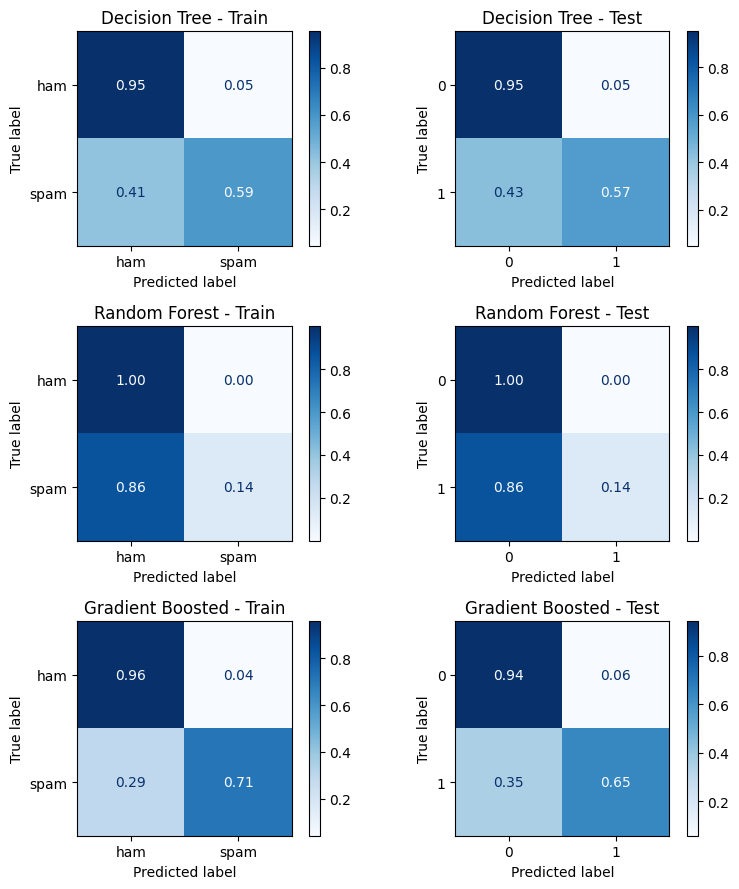
models = [
    ('Decision Tree', y_tree_train, y_tree_test),
    ('Random Forest', y_forest_train, y_forest_test),
    ('Gradient Boosted', y_boosted_train, y_boosted_test)
]

fig, axes = plt.subplots(3, 2, figsize=(8, 9))

for i, (name, y_pred_train, y_pred_test) in enumerate(models):
    cm_train = confusion_matrix(y_train, y_pred_train, normalize = 'true')
    cm_test = confusion_matrix(y_test, y_pred_test, normalize = 'true')

    disp_train = ConfusionMatrixDisplay(cm_train, display_labels=labels)
    disp_test = ConfusionMatrixDisplay(cm_test)

    disp_train.plot(ax=axes[i, 0], cmap='Blues', values_format='.2f')
    axes[i, 0].set_title(f'{name} - Train')

    disp_test.plot(ax=axes[i, 1], cmap='Blues', values_format='.2f')
    axes[i, 1].set_title(f'{name} - Test')

plt.tight_layout()