
Pandas Refresher#
In your first problem set, you’ll be using the King County Housing dataset. This dataset contains information about the sales of residences (homes, condos, apartment buildings) within King County, WA (the county containing Seattle) from the 2014-2015 period.
import pandas as pd
import matplotlib.pyplot as plt
import numpy as np
housing_df = pd.read_csv('https://raw.githubusercontent.com/GettysburgDataScience/datasets/refs/heads/main/kc_house_data.csv', parse_dates = ['date'])
housing_df['day'] = housing_df['date'].dt.day
housing_df['month'] = housing_df['date'].dt.month
housing_df['year'] = housing_df['date'].dt.year
housing_df.info()
<class 'pandas.core.frame.DataFrame'>
RangeIndex: 21613 entries, 0 to 21612
Data columns (total 24 columns):
 #   Column         Non-Null Count  Dtype
---  ------         --------------  -----
 0   id             21613 non-null  int64
 1   date           21613 non-null  datetime64[ns]
 2   price          21613 non-null  float64
 3   bedrooms       21613 non-null  int64
 4   bathrooms      21613 non-null  float64
 5   sqft_living    21613 non-null  int64
 6   sqft_lot       21613 non-null  int64
 7   floors         21613 non-null  float64
 8   waterfront     21613 non-null  int64
 9   view           21613 non-null  int64
 10  condition      21613 non-null  int64
 11  grade          21613 non-null  int64
 12  sqft_above     21613 non-null  int64
 13  sqft_basement  21613 non-null  int64
 14  yr_built       21613 non-null  int64
 15  yr_renovated   21613 non-null  int64
 16  zipcode        21613 non-null  int64
 17  lat            21613 non-null  float64
 18  long           21613 non-null  float64
 19  sqft_living15  21613 non-null  int64
 20  sqft_lot15     21613 non-null  int64
 21  day            21613 non-null  int32
 22  month          21613 non-null  int32
 23  year           21613 non-null  int32
dtypes: datetime64[ns](1), float64(5), int32(3), int64(15)
memory usage: 3.7 MB
housing_df[['date', 'day', 'month', 'year']]
| date | day | month | year | |
|---|---|---|---|---|
| 0 | 2014-10-13 | 13 | 10 | 2014 |
| 1 | 2014-12-09 | 9 | 12 | 2014 |
| 2 | 2015-02-25 | 25 | 2 | 2015 |
| 3 | 2014-12-09 | 9 | 12 | 2014 |
| 4 | 2015-02-18 | 18 | 2 | 2015 |
| ... | ... | ... | ... | ... |
| 21608 | 2014-05-21 | 21 | 5 | 2014 |
| 21609 | 2015-02-23 | 23 | 2 | 2015 |
| 21610 | 2014-06-23 | 23 | 6 | 2014 |
| 21611 | 2015-01-16 | 16 | 1 | 2015 |
| 21612 | 2014-10-15 | 15 | 10 | 2014 |
21613 rows × 4 columns
Finding information#
Google - Better than ChatGPT for most things and only 10% of the energy consumption on a query basis. THINK OF THE TREES!
DuckDuckGo - Like Google but without storing and using your data.
Common Pandas Functions#
Data Exploration#
head() - Returns the first n rows of a DataFrame (default is 5 rows). Useful for quickly previewing data.
tail() - Returns the last n rows of a DataFrame (default is 5 rows). Helpful for checking the end of your dataset.
info() - Displays a concise summary of a DataFrame, including column names, data types, non-null counts, and memory usage.
describe() - Generates descriptive statistics for numerical columns (count, mean, std, min, 25%, 50%, 75%, max).
unique() - Returns unique values.
Data Selection and Filtering#
Data Cleaning#
Data Transformation and Aggregation#
groupby() - Groups DataFrame rows by one or more columns, enabling aggregation and analysis by group.
agg() - Applies one or more aggregation functions to DataFrame columns, often used with
groupby()for grouped statistics.apply() - Applies a custom function along an axis of the DataFrame (row-wise or column-wise), enabling flexible data transformations.
sort_values() - Sorts DataFrame rows by one or more columns.
value_counts() - Returns counts of unique values, useful for categorical analysis.
Data Combining#
Visualization#
This chart may help you decide on how you would want to visualize your data. Then, visit Matplotlib Gallery, find the type of chart you want to make and template your code based on the examples.
Together Questions#
How many listings are recorded in this dataframe?
How many of them have between 2-5 bedrooms and 1+ bathrooms?
I’m looking for a house with 3-5 bedrooms and 2+ bathrooms. Where should I look?
What can I expect to pay for a 1500 sq ft house in this neighborhood?
Practice Questions#
Think before you code. For each problem below, discuss the steps you would take and find the corresponding functions. Write out your plan in the markdown cell with the question.
1
What is the range of values for number of bedrooms, number of bathrooms, and square footage?
If we were only interested in single family homes, how might you filter the dataset?
2
How many houses were sold for more than $500,000?
What is the average price of houses with 3 or more bedrooms?
3
What is the average price per number of bedrooms?
What is the average price per number of bedrooms for each zip code? How would you effectively convey this information?
4
Create a plot that conveys some difference (your choice) between zip codes (e.g. price/sq ft, number of houses sold, lot size, grade).
The plot(s) should show the spatial relationship between zip codes with only one data point per zip code (that is, you’re not displaying individual sales).
5
House flippers buy houses in need of repair/renovation, fix them up quickly, and resell them. Identify sales that would have been good candidates for flipping.
Consider, the house doesn’t have to be cheap, it just has to have the potential to sell for more. How do you quantify that?
Create a graphic for prospective home flippers. What information would be useful for them to know? How would you show that?
6
Think of a particular audience (e.g. home seller, home buyer, real estate agent, etc) and identify a question or want they may have. Create a graphic to address that question/want.
def quantize(data, bin_width):
    return bin_width * (data//bin_width)
housing_df['long_r'] = quantize(housing_df['long'], 0.05)
housing_df['lat_r'] = quantize(housing_df['lat'], 0.05)
housing_df.groupby(by = ['long_r', 'lat_r']).agg({'price_per_sqft':'median'})
---------------------------------------------------------------------------
KeyError                                  Traceback (most recent call last)
Cell In[7], line 1
----> 1 housing_df.groupby(by = ['long_r', 'lat_r']).agg({'price_per_sqft':'median'})

File ~/.pyenv/versions/3.13.1/envs/datascience/lib/python3.13/site-packages/pandas/core/groupby/generic.py:1432, in DataFrameGroupBy.aggregate(self, func, engine, engine_kwargs, *args, **kwargs)
   1429     kwargs["engine_kwargs"] = engine_kwargs
   1431 op = GroupByApply(self, func, args=args, kwargs=kwargs)
-> 1432 result = op.agg()
   1433 if not is_dict_like(func) and result is not None:
   1434     # GH #52849
   1435     if not self.as_index and is_list_like(func):

File ~/.pyenv/versions/3.13.1/envs/datascience/lib/python3.13/site-packages/pandas/core/apply.py:190, in Apply.agg(self)
    187     return self.apply_str()
    189 if is_dict_like(func):
--> 190     return self.agg_dict_like()
    191 elif is_list_like(func):
    192     # we require a list, but not a 'str'
    193     return self.agg_list_like()

File ~/.pyenv/versions/3.13.1/envs/datascience/lib/python3.13/site-packages/pandas/core/apply.py:423, in Apply.agg_dict_like(self)
    415 def agg_dict_like(self) -> DataFrame | Series:
    416     """
    417     Compute aggregation in the case of a dict-like argument.
    418
   (...)    421     Result of aggregation.
    422     """
--> 423     return self.agg_or_apply_dict_like(op_name="agg")

File ~/.pyenv/versions/3.13.1/envs/datascience/lib/python3.13/site-packages/pandas/core/apply.py:1603, in GroupByApply.agg_or_apply_dict_like(self, op_name)
   1598     kwargs.update({"engine": engine, "engine_kwargs": engine_kwargs})
   1600 with com.temp_setattr(
   1601     obj, "as_index", True, condition=hasattr(obj, "as_index")
   1602 ):
-> 1603     result_index, result_data = self.compute_dict_like(
   1604         op_name, selected_obj, selection, kwargs
   1605     )
   1606 result = self.wrap_results_dict_like(selected_obj, result_index, result_data)
   1607 return result

File ~/.pyenv/versions/3.13.1/envs/datascience/lib/python3.13/site-packages/pandas/core/apply.py:462, in Apply.compute_dict_like(self, op_name, selected_obj, selection, kwargs)
    460 is_groupby = isinstance(obj, (DataFrameGroupBy, SeriesGroupBy))
    461 func = cast(AggFuncTypeDict, self.func)
--> 462 func = self.normalize_dictlike_arg(op_name, selected_obj, func)
    464 is_non_unique_col = (
    465     selected_obj.ndim == 2
    466     and selected_obj.columns.nunique() < len(selected_obj.columns)
    467 )
    469 if selected_obj.ndim == 1:
    470     # key only used for output

File ~/.pyenv/versions/3.13.1/envs/datascience/lib/python3.13/site-packages/pandas/core/apply.py:663, in Apply.normalize_dictlike_arg(self, how, obj, func)
    661     cols = Index(list(func.keys())).difference(obj.columns, sort=True)
    662     if len(cols) > 0:
--> 663         raise KeyError(f"Column(s) {list(cols)} do not exist")
    665 aggregator_types = (list, tuple, dict)
    667 # if we have a dict of any non-scalars
    668 # eg. {'A' : ['mean']}, normalize all to
    669 # be list-likes
    670 # Cannot use func.values() because arg may be a Series

KeyError: "Column(s) ['price_per_sqft'] do not exist"
housing_df['price_per_sqft'] = housing_df['price']/housing_df['sqft_living']
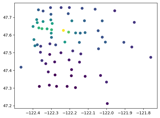
zip_price = housing_df.groupby(by='zipcode').agg({'price_per_sqft':'median', 'lat':'mean', 'long':'mean'}).sort_values(by='price_per_sqft', ascending=False)
zip_price.head()
| price_per_sqft | lat | long | |
|---|---|---|---|
| zipcode | |||
| 98039 | 565.165614 | 47.625840 | -122.233540 |
| 98004 | 456.944444 | 47.616183 | -122.205189 |
| 98109 | 427.696078 | 47.635602 | -122.350092 |
| 98112 | 423.828125 | 47.629619 | -122.297866 |
| 98119 | 416.652778 | 47.640034 | -122.366918 |
plt.scatter(zip_price['long'], zip_price['lat'], c = zip_price['price_per_sqft'])
plt.show()
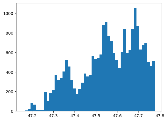
plt.hist(housing_df['lat'], bins = 50)
plt.show()
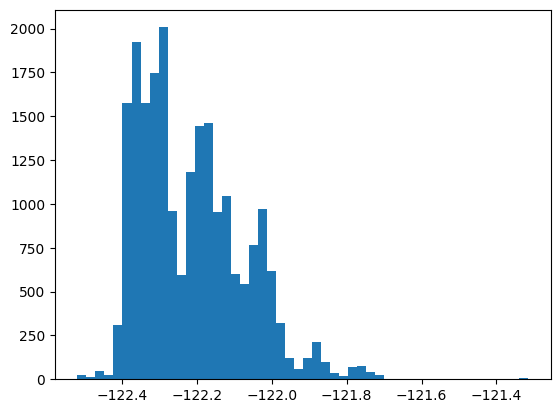
plt.hist(housing_df['long'], bins = 50)
plt.show()
import seaborn as sns
s = sns.jointplot(x='long', y='lat', hue = 'price_per_sqft', data = housing_df, kind = 'hist')
s.ax_joint.grid(False)
s.ax_marg_y.grid(False)
s.fig.suptitle("Sales by firm's age")
---------------------------------------------------------------------------
KeyboardInterrupt                         Traceback (most recent call last)
Cell In[10], line 2
      1 import seaborn as sns
----> 2 s = sns.jointplot(x='long', y='lat', hue = 'price_per_sqft', data = housing_df, kind = 'hist')
      3 s.ax_joint.grid(False)
      4 s.ax_marg_y.grid(False)

File ~/.pyenv/versions/3.13.1/envs/datascience/lib/python3.13/site-packages/seaborn/axisgrid.py:2275, in jointplot(data, x, y, hue, kind, height, ratio, space, dropna, xlim, ylim, color, palette, hue_order, hue_norm, marginal_ticks, joint_kws, marginal_kws, **kwargs)
   2269 elif kind.startswith("hist"):
   2270
   2271     # TODO process pair parameters for bins, etc. and pass
   2272     # to both joint and marginal plots
   2274     joint_kws.setdefault("color", color)
-> 2275     grid.plot_joint(histplot, **joint_kws)
   2277     marginal_kws.setdefault("kde", False)
   2278     marginal_kws.setdefault("color", color)

File ~/.pyenv/versions/3.13.1/envs/datascience/lib/python3.13/site-packages/seaborn/axisgrid.py:1832, in JointGrid.plot_joint(self, func, **kwargs)
   1829     self._inject_kwargs(func, kwargs, self._hue_params)
   1831 if str(func.__module__).startswith("seaborn"):
-> 1832     func(x=self.x, y=self.y, **kwargs)
   1833 else:
   1834     func(self.x, self.y, **kwargs)

File ~/.pyenv/versions/3.13.1/envs/datascience/lib/python3.13/site-packages/seaborn/distributions.py:1434, in histplot(data, x, y, hue, weights, stat, bins, binwidth, binrange, discrete, cumulative, common_bins, common_norm, multiple, element, fill, shrink, kde, kde_kws, line_kws, thresh, pthresh, pmax, cbar, cbar_ax, cbar_kws, palette, hue_order, hue_norm, color, log_scale, legend, ax, **kwargs)
   1416     p.plot_univariate_histogram(
   1417         multiple=multiple,
   1418         element=element,
   (...)   1429         **kwargs,
   1430     )
   1432 else:
-> 1434     p.plot_bivariate_histogram(
   1435         common_bins=common_bins,
   1436         common_norm=common_norm,
   1437         thresh=thresh,
   1438         pthresh=pthresh,
   1439         pmax=pmax,
   1440         color=color,
   1441         legend=legend,
   1442         cbar=cbar,
   1443         cbar_ax=cbar_ax,
   1444         cbar_kws=cbar_kws,
   1445         estimate_kws=estimate_kws,
   1446         **kwargs,
   1447     )
   1449 return ax

File ~/.pyenv/versions/3.13.1/envs/datascience/lib/python3.13/site-packages/seaborn/distributions.py:850, in _DistributionPlotter.plot_bivariate_histogram(self, common_bins, common_norm, thresh, pthresh, pmax, color, legend, cbar, cbar_ax, cbar_kws, estimate_kws, **plot_kws)
    846     heights = np.ma.masked_less_equal(heights, thresh)
    848 # pcolormesh is going to turn the grid off, but we want to keep it
    849 # I'm not sure if there's a better way to get the grid state
--> 850 x_grid = any([l.get_visible() for l in ax.xaxis.get_gridlines()])
    851 y_grid = any([l.get_visible() for l in ax.yaxis.get_gridlines()])
    853 mesh = ax.pcolormesh(
    854     x_edges,
    855     y_edges,
    856     heights.T,
    857     **artist_kws,
    858 )

File ~/.pyenv/versions/3.13.1/envs/datascience/lib/python3.13/site-packages/matplotlib/axis.py:1423, in Axis.get_gridlines(self)
   1421 def get_gridlines(self):
   1422     r"""Return this Axis' grid lines as a list of `.Line2D`\s."""
-> 1423     ticks = self.get_major_ticks()
   1424     return cbook.silent_list('Line2D gridline',
   1425                              [tick.gridline for tick in ticks])

File ~/.pyenv/versions/3.13.1/envs/datascience/lib/python3.13/site-packages/matplotlib/axis.py:1660, in Axis.get_major_ticks(self, numticks)
   1645 r"""
   1646 Return the list of major `.Tick`\s.
   1647
   (...)   1657     Use `.set_tick_params` instead if possible.
   1658 """
   1659 if numticks is None:
-> 1660     numticks = len(self.get_majorticklocs())
   1662 while len(self.majorTicks) < numticks:
   1663     # Update the new tick label properties from the old.
   1664     tick = self._get_tick(major=True)

File ~/.pyenv/versions/3.13.1/envs/datascience/lib/python3.13/site-packages/matplotlib/axis.py:1525, in Axis.get_majorticklocs(self)
   1523 def get_majorticklocs(self):
   1524     """Return this Axis' major tick locations in data coordinates."""
-> 1525     return self.major.locator()

File ~/.pyenv/versions/3.13.1/envs/datascience/lib/python3.13/site-packages/matplotlib/ticker.py:2229, in MaxNLocator.__call__(self)
   2228 def __call__(self):
-> 2229     vmin, vmax = self.axis.get_view_interval()
   2230     return self.tick_values(vmin, vmax)

File ~/.pyenv/versions/3.13.1/envs/datascience/lib/python3.13/site-packages/matplotlib/axis.py:2347, in _make_getset_interval.<locals>.getter(self)
   2345 def getter(self):
   2346     # docstring inherited.
-> 2347     return getattr(getattr(self.axes, lim_name), attr_name)

File ~/.pyenv/versions/3.13.1/envs/datascience/lib/python3.13/site-packages/matplotlib/axes/_base.py:904, in _AxesBase.viewLim(self)
    901 @property
    902 def viewLim(self):
    903     """The view limits as `.Bbox` in data coordinates."""
--> 904     self._unstale_viewLim()
    905     return self._viewLim

File ~/.pyenv/versions/3.13.1/envs/datascience/lib/python3.13/site-packages/matplotlib/axes/_base.py:898, in _AxesBase._unstale_viewLim(self)
    896     for ax in self._shared_axes[name].get_siblings(self):
    897         ax._stale_viewlims[name] = False
--> 898 self.autoscale_view(**{f"scale{name}": scale
    899                        for name, scale in need_scale.items()})

File ~/.pyenv/versions/3.13.1/envs/datascience/lib/python3.13/site-packages/matplotlib/axes/_base.py:3012, in _AxesBase.autoscale_view(self, tight, scalex, scaley)
   3007         x_stickies = np.sort(np.concatenate([
   3008             artist.sticky_edges.x
   3009             for ax in self._shared_axes["x"].get_siblings(self)
   3010             for artist in ax.get_children()]))
   3011     if self._ymargin and scaley and self.get_autoscaley_on():
-> 3012         y_stickies = np.sort(np.concatenate([
   3013             artist.sticky_edges.y
   3014             for ax in self._shared_axes["y"].get_siblings(self)
   3015             for artist in ax.get_children()]))
   3016 if self.get_xscale() == 'log':
   3017     x_stickies = x_stickies[x_stickies > 0]

KeyboardInterrupt: