2.3. Example: Simple Linear Regression with the King County Housing Dataset#
In your second problem set, you’ll be using the King County Housing dataset. This dataset contains information about the sales of residences (homes, condos, apartment buildings) within King County, WA (the county containing Seattle) from the 2014-2015 period.
import pandas as pd
import matplotlib.pyplot as plt
import numpy as np
housing_df = pd.read_csv('https://raw.githubusercontent.com/GettysburgDataScience/datasets/refs/heads/main/kc_house_data.csv', parse_dates = ['date'])
housing_df.info()
<class 'pandas.core.frame.DataFrame'>
RangeIndex: 21613 entries, 0 to 21612
Data columns (total 21 columns):
 #   Column         Non-Null Count  Dtype
---  ------         --------------  -----
 0   id             21613 non-null  int64
 1   date           21613 non-null  datetime64[ns]
 2   price          21613 non-null  float64
 3   bedrooms       21613 non-null  int64
 4   bathrooms      21613 non-null  float64
 5   sqft_living    21613 non-null  int64
 6   sqft_lot       21613 non-null  int64
 7   floors         21613 non-null  float64
 8   waterfront     21613 non-null  int64
 9   view           21613 non-null  int64
 10  condition      21613 non-null  int64
 11  grade          21613 non-null  int64
 12  sqft_above     21613 non-null  int64
 13  sqft_basement  21613 non-null  int64
 14  yr_built       21613 non-null  int64
 15  yr_renovated   21613 non-null  int64
 16  zipcode        21613 non-null  int64
 17  lat            21613 non-null  float64
 18  long           21613 non-null  float64
 19  sqft_living15  21613 non-null  int64
 20  sqft_lot15     21613 non-null  int64
dtypes: datetime64[ns](1), float64(5), int64(15)
memory usage: 3.5 MB
housing_df.head()
| id | date | price | bedrooms | bathrooms | sqft_living | sqft_lot | floors | waterfront | view | ... | grade | sqft_above | sqft_basement | yr_built | yr_renovated | zipcode | lat | long | sqft_living15 | sqft_lot15 | |
|---|---|---|---|---|---|---|---|---|---|---|---|---|---|---|---|---|---|---|---|---|---|
| 0 | 7129300520 | 2014-10-13 | 221900.0 | 3 | 1.00 | 1180 | 5650 | 1.0 | 0 | 0 | ... | 7 | 1180 | 0 | 1955 | 0 | 98178 | 47.5112 | -122.257 | 1340 | 5650 |
| 1 | 6414100192 | 2014-12-09 | 538000.0 | 3 | 2.25 | 2570 | 7242 | 2.0 | 0 | 0 | ... | 7 | 2170 | 400 | 1951 | 1991 | 98125 | 47.7210 | -122.319 | 1690 | 7639 |
| 2 | 5631500400 | 2015-02-25 | 180000.0 | 2 | 1.00 | 770 | 10000 | 1.0 | 0 | 0 | ... | 6 | 770 | 0 | 1933 | 0 | 98028 | 47.7379 | -122.233 | 2720 | 8062 |
| 3 | 2487200875 | 2014-12-09 | 604000.0 | 4 | 3.00 | 1960 | 5000 | 1.0 | 0 | 0 | ... | 7 | 1050 | 910 | 1965 | 0 | 98136 | 47.5208 | -122.393 | 1360 | 5000 |
| 4 | 1954400510 | 2015-02-18 | 510000.0 | 3 | 2.00 | 1680 | 8080 | 1.0 | 0 | 0 | ... | 8 | 1680 | 0 | 1987 | 0 | 98074 | 47.6168 | -122.045 | 1800 | 7503 |
5 rows × 21 columns
2.3.1. Linear Regression#
2.3.1.1. Narrowing the scope of the problem#
For this example, we’ll filter the dataset only to 3 BR homes in a single zip code. And, for the sake of having enough data, we’ll use the zip code with the greatest number of 3 BR homes sold, which is 98042.
So you might imagine that you’re trying to sell your 3 BR home in 98042, and you want to estimate what a fair market price would be and set your asking price accordingly.
# Finding the zip code with the most 3 BR homes

housing_df.query('bedrooms==3')\
    .groupby(by = 'zipcode').agg({'id':'count'})\
        .sort_values(by='id', ascending = False)
| id | |
|---|---|
| zipcode | |
| 98042 | 317 |
| 98034 | 303 |
| 98038 | 292 |
| 98103 | 283 |
| 98023 | 281 |
| ... | ... |
| 98010 | 51 |
| 98102 | 51 |
| 98024 | 44 |
| 98148 | 34 |
| 98039 | 11 |
70 rows × 1 columns
# Filtering the data to only include 3 BR homes in that zip code.

housing3 = housing_df.query('bedrooms == 3 and zipcode == 98042')
housing3
| id | date | price | bedrooms | bathrooms | sqft_living | sqft_lot | floors | waterfront | view | ... | grade | sqft_above | sqft_basement | yr_built | yr_renovated | zipcode | lat | long | sqft_living15 | sqft_lot15 | |
|---|---|---|---|---|---|---|---|---|---|---|---|---|---|---|---|---|---|---|---|---|---|
| 57 | 2799800710 | 2015-04-07 | 301000.0 | 3 | 2.50 | 2420 | 4750 | 2.0 | 0 | 0 | ... | 8 | 2420 | 0 | 2003 | 0 | 98042 | 47.3663 | -122.122 | 2690 | 4750 |
| 68 | 1274500060 | 2014-08-25 | 204000.0 | 3 | 1.00 | 1000 | 12070 | 1.0 | 0 | 0 | ... | 7 | 1000 | 0 | 1968 | 0 | 98042 | 47.3621 | -122.110 | 1010 | 12635 |
| 74 | 3444100400 | 2015-03-16 | 349000.0 | 3 | 1.75 | 1790 | 50529 | 1.0 | 0 | 0 | ... | 7 | 1090 | 700 | 1965 | 0 | 98042 | 47.3511 | -122.073 | 1940 | 50529 |
| 201 | 2222059065 | 2014-11-12 | 297000.0 | 3 | 2.50 | 1940 | 14952 | 2.0 | 0 | 0 | ... | 8 | 1940 | 0 | 1994 | 0 | 98042 | 47.3777 | -122.165 | 2030 | 10450 |
| 296 | 5468730030 | 2014-08-22 | 265000.0 | 3 | 2.00 | 1320 | 8959 | 1.0 | 0 | 0 | ... | 7 | 1320 | 0 | 1993 | 0 | 98042 | 47.3536 | -122.144 | 1740 | 7316 |
| ... | ... | ... | ... | ... | ... | ... | ... | ... | ... | ... | ... | ... | ... | ... | ... | ... | ... | ... | ... | ... | ... |
| 21420 | 9478550110 | 2015-03-03 | 299950.0 | 3 | 2.50 | 1740 | 4497 | 2.0 | 0 | 0 | ... | 7 | 1740 | 0 | 2012 | 0 | 98042 | 47.3697 | -122.117 | 1950 | 4486 |
| 21451 | 7140700690 | 2015-03-12 | 239950.0 | 3 | 1.75 | 1600 | 4888 | 1.0 | 0 | 0 | ... | 6 | 1600 | 0 | 2014 | 0 | 98042 | 47.3830 | -122.097 | 2520 | 5700 |
| 21526 | 1760650820 | 2015-04-28 | 290000.0 | 3 | 2.25 | 1610 | 3764 | 2.0 | 0 | 0 | ... | 7 | 1610 | 0 | 2012 | 0 | 98042 | 47.3589 | -122.083 | 1610 | 3825 |
| 21553 | 2522059251 | 2015-04-09 | 465000.0 | 3 | 2.50 | 2050 | 15035 | 2.0 | 0 | 0 | ... | 9 | 2050 | 0 | 2006 | 0 | 98042 | 47.3619 | -122.122 | 1300 | 15836 |
| 21585 | 3832050760 | 2014-08-28 | 270000.0 | 3 | 2.50 | 1870 | 5000 | 2.0 | 0 | 0 | ... | 7 | 1870 | 0 | 2009 | 0 | 98042 | 47.3339 | -122.055 | 2170 | 5399 |
317 rows × 21 columns
2.3.1.2. Cleaning the data and selecting a feature#
We’ll remove columns that are either uninformative (e.g. id, date) or constant (e.g. bedrooms, zipcode, waterfront).
I like to do this by:
requesting all the columns
copying all the columns into a list (columns_to_keep)
removing the ones I want removed
extracting just those columns from the dataframe
housing3.columns
Index(['id', 'date', 'price', 'bedrooms', 'bathrooms', 'sqft_living',
       'sqft_lot', 'floors', 'waterfront', 'view', 'condition', 'grade',
       'sqft_above', 'sqft_basement', 'yr_built', 'yr_renovated', 'zipcode',
       'lat', 'long', 'sqft_living15', 'sqft_lot15'],
      dtype='object')
columns_to_keep = ['price', 'bathrooms', 'sqft_living',
       'sqft_lot', 'floors', 'condition', 'grade',
       'sqft_above', 'sqft_basement', 'yr_built', 'yr_renovated',
       'lat', 'long', 'sqft_living15', 'sqft_lot15']

housing3 = housing3[columns_to_keep]
Next, we’ll calculate the correlation and display it as a heat map. We’ll select the variable most correlated to price as our feature for modeling.
housing_corr = housing3.corr()
housing_corr
| price | bathrooms | sqft_living | sqft_lot | floors | condition | grade | sqft_above | sqft_basement | yr_built | yr_renovated | lat | long | sqft_living15 | sqft_lot15 | |
|---|---|---|---|---|---|---|---|---|---|---|---|---|---|---|---|
| price | 1.000000 | 0.545442 | 0.809535 | 0.540426 | 0.394416 | -0.161509 | 0.725263 | 0.797889 | 0.048380 | 0.310763 | -0.029596 | -0.009834 | -0.161651 | 0.661501 | 0.417028 |
| bathrooms | 0.545442 | 1.000000 | 0.700860 | 0.080940 | 0.644609 | -0.431470 | 0.533476 | 0.685417 | 0.055520 | 0.707861 | -0.162385 | 0.133747 | -0.192372 | 0.610515 | 0.118165 |
| sqft_living | 0.809535 | 0.700860 | 1.000000 | 0.284833 | 0.522319 | -0.307134 | 0.734776 | 0.923458 | 0.217862 | 0.432447 | -0.112420 | 0.036043 | -0.241881 | 0.770141 | 0.265556 |
| sqft_lot | 0.540426 | 0.080940 | 0.284833 | 1.000000 | 0.019590 | -0.013589 | 0.136916 | 0.230406 | 0.145040 | -0.123200 | 0.138612 | 0.019995 | -0.016856 | 0.238468 | 0.562668 |
| floors | 0.394416 | 0.644609 | 0.522319 | 0.019590 | 1.000000 | -0.409100 | 0.403710 | 0.639940 | -0.287080 | 0.632382 | -0.117929 | 0.009782 | -0.157313 | 0.488257 | -0.021495 |
| condition | -0.161509 | -0.431470 | -0.307134 | -0.013589 | -0.409100 | 1.000000 | -0.201157 | -0.297693 | -0.031132 | -0.504516 | -0.113069 | -0.000707 | 0.147085 | -0.362378 | -0.010971 |
| grade | 0.725263 | 0.533476 | 0.734776 | 0.136916 | 0.403710 | -0.201157 | 1.000000 | 0.751795 | -0.026266 | 0.337224 | -0.164262 | -0.016369 | -0.264209 | 0.690822 | 0.092479 |
| sqft_above | 0.797889 | 0.685417 | 0.923458 | 0.230406 | 0.639940 | -0.297693 | 0.751795 | 1.000000 | -0.173297 | 0.480472 | -0.119714 | -0.004595 | -0.237341 | 0.740524 | 0.165258 |
| sqft_basement | 0.048380 | 0.055520 | 0.217862 | 0.145040 | -0.287080 | -0.031132 | -0.026266 | -0.173297 | 1.000000 | -0.112136 | 0.015948 | 0.104201 | -0.017151 | 0.093178 | 0.261271 |
| yr_built | 0.310763 | 0.707861 | 0.432447 | -0.123200 | 0.632382 | -0.504516 | 0.337224 | 0.480472 | -0.112136 | 1.000000 | -0.175139 | -0.010309 | -0.036663 | 0.488356 | -0.109969 |
| yr_renovated | -0.029596 | -0.162385 | -0.112420 | 0.138612 | -0.117929 | -0.113069 | -0.164262 | -0.119714 | 0.015948 | -0.175139 | 1.000000 | -0.038023 | 0.093257 | -0.113313 | 0.157284 |
| lat | -0.009834 | 0.133747 | 0.036043 | 0.019995 | 0.009782 | -0.000707 | -0.016369 | -0.004595 | 0.104201 | -0.010309 | -0.038023 | 1.000000 | -0.430948 | 0.073604 | -0.081197 |
| long | -0.161651 | -0.192372 | -0.241881 | -0.016856 | -0.157313 | 0.147085 | -0.264209 | -0.237341 | -0.017151 | -0.036663 | 0.093257 | -0.430948 | 1.000000 | -0.237247 | -0.030228 |
| sqft_living15 | 0.661501 | 0.610515 | 0.770141 | 0.238468 | 0.488257 | -0.362378 | 0.690822 | 0.740524 | 0.093178 | 0.488356 | -0.113313 | 0.073604 | -0.237247 | 1.000000 | 0.092127 |
| sqft_lot15 | 0.417028 | 0.118165 | 0.265556 | 0.562668 | -0.021495 | -0.010971 | 0.092479 | 0.165258 | 0.261271 | -0.109969 | 0.157284 | -0.081197 | -0.030228 | 0.092127 | 1.000000 |
import seaborn as sns
fig, ax = plt.subplots(1,1, figsize = (8,8))

sns.heatmap(np.abs(housing_corr), vmin = 0, vmax = 1,
            annot = True, annot_kws = {'size':8},
            cbar = False)
plt.show()
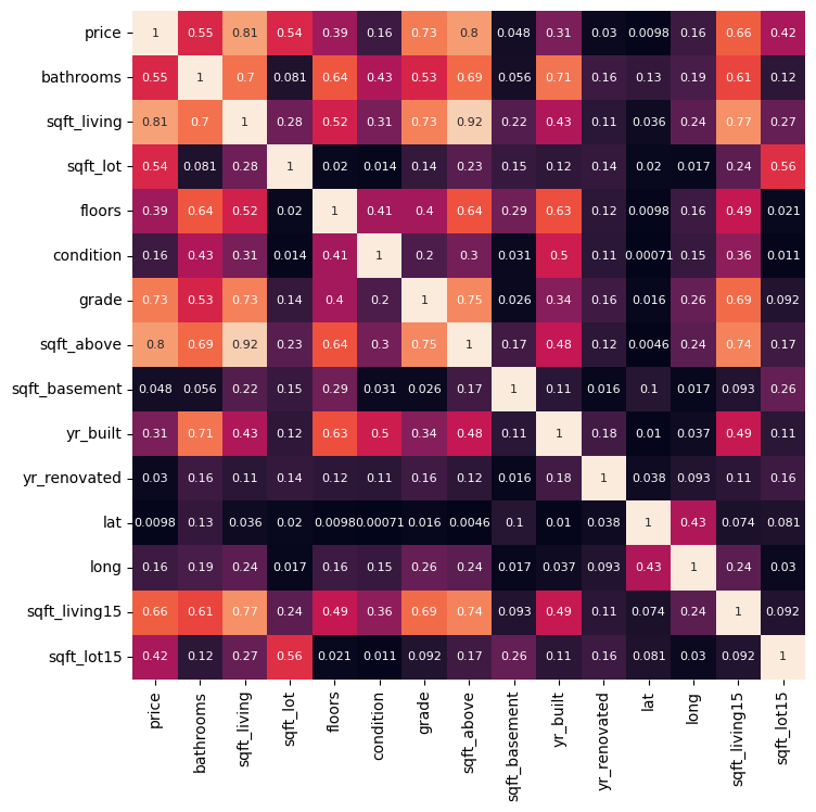
With a correlation of 0.81, sqft_living is most correlated to price. So:
sqft_living is our feature
price is our target
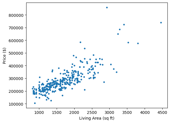
Let’s plot price vs sqft_living to see our dataset.
x = housing3[['sqft_living']]
y = housing3[['price']]

plt.plot(x, y, '.')
plt.xlabel('Living Area (sq ft)')
plt.ylabel('Price ($)')
plt.show()
2.3.1.3. Modeling time!#
We will:
Import the necessary functions
Split our data into training and testing sets
Create our model template, LinearRegression()
Fit our model to the training data.
Make predictions using both our training and testing data.
Calculate \(R^2\) and RMSE for both training and testing sets.
Visualize our results.
# Importing packages

import sklearn as sk

from sklearn.linear_model import LinearRegression
from sklearn.model_selection import train_test_split
from sklearn.datasets import make_regression
from sklearn.metrics import root_mean_squared_error, r2_score
# Splitting the data
x_train, x_test, y_train, y_test = train_test_split(x, y, test_size = 0.2, random_state=13)
# Creating and fitting the model
linreg = LinearRegression()  #makes the template
linreg.fit(x_train, y_train) #finds the optimal slope and
LinearRegression()In a Jupyter environment, please rerun this cell to show the HTML representation or trust the notebook.
On GitHub, the HTML representation is unable to render, please try loading this page with nbviewer.org.
Parameters
| fit_intercept | True | |
| copy_X | True | |
| tol | 1e-06 | |
| n_jobs | None | |
| positive | False |
x_model = np.array([[0, 4500]]).T
y_model = linreg.predict(x_model)

plt.plot(x, y, '.', alpha = 0.8)
plt.plot(x_model, y_model, 'k--', label = 'Best-fit line')

plt.title('Predicting Sale Price from Living Area')
plt.xlabel('Living Area (sq ft)')
plt.ylabel('Price ($)')
plt.show()
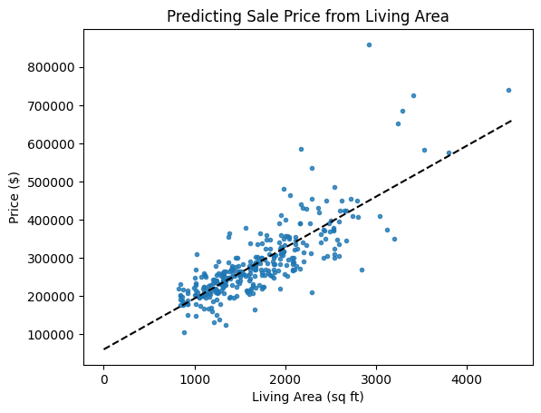
What do you think of the fit of this line? I see an issue…
This fit is okay and I won’t change it, but something bothers me. Do you see it? What could be done to improve the fit?
# Inspecting the model parameters
linreg.__dict__
{'fit_intercept': True,
 'copy_X': True,
 'tol': 1e-06,
 'n_jobs': None,
 'positive': False,
 'feature_names_in_': array(['sqft_living'], dtype=object),
 'n_features_in_': 1,
 'coef_': array([[133.30980501]]),
 'rank_': 1,
 'singular_': array([9115.35178206]),
 'intercept_': array([60720.98693839])}
Do you see the slope and y-intercept in the list of model properties above?
slope = 133.31 ($/sqft)
y-intercept = 60,720.99 ($)
2.3.1.4. Assessing the model#
# Use the training and testing features to make predictions using the model
y_pred_train = linreg.predict(x_train)
y_pred_test = linreg.predict(x_test)
# Calculate R2
r2_train = r2_score(y_train, y_pred_train)
r2_test = r2_score(y_test, y_pred_test)

# Calculate RMSE
rmse_train = root_mean_squared_error(y_train, y_pred_train)
rmse_test = root_mean_squared_error(y_test, y_pred_test)

print(f'R2 train: {r2_train:.2f}\t\tRMSE train: {rmse_train:.2f}')
print(f'R2 test: {r2_test:.2f}\t\tRMSE test: {rmse_test:.2f}')
R2 train: 0.66		RMSE train: 55145.81
R2 test: 0.65		RMSE test: 62150.55
Why do we assess model performance on both training and testing data?
We’ll talk more about model fit later, but what we want to see: similar performance between training and testing results, but testing is generally slightly worse.
If the model does well with training data and much worse with test data, this typically indicates over-fitting and you probably need a simpler model or more data. We are using as simple a model as possible, so that’s not an issue.
If the model does badly with both training and testing data, this indicates under-fitting, and we could probably use a better model (more parameters).
Sometimes, depending on the random sampling of the train-test split, you may even get better performance on the testing data. This only really happens with smaller data sets such as this.
2.3.1.5. Another Visualization#
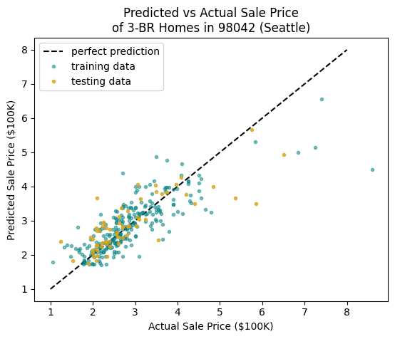
We can also visualize the predicted vs actual values. Later, when we use more features in our model, this is our only good option.
This plot helps visualize where the model is over-estimating or under-estimating the prices of homes. A point below the line means the actual price is greater than the predicted price, so the model is under-estimating; a point above suggests the model is over-estimating.
Do you see a problem now?
# I will divide prices by 100K saved as variable HK
HK = 100000
low, high = 1, 8

plt.plot([low, high], [low, high], 'k--', label = 'perfect prediction')

# plot the training data
plt.plot(y_train/HK, y_pred_train/HK,
         '.', color = 'teal', alpha = 0.5,
         label = 'training data')

# plot the test data
plt.plot(y_test/HK, y_pred_test/HK,
         '.', color = 'goldenrod', alpha = 0.8,
         label = 'testing data')

plt.title('Predicted vs Actual Sale Price\nof 3-BR Homes in 98042 (Seattle)')
plt.xlabel('Actual Sale Price ($100K)')
plt.ylabel('Predicted Sale Price ($100K)')
plt.legend()
plt.show()