2.4. Example: Multiple Linear Regression Estimating Fuel Efficiency

import pandas as pd
import numpy as np
import matplotlib.pyplot as plt
import seaborn as sns

data_df = pd.read_csv('https://raw.githubusercontent.com/shreyamdg/automobile-data-set-analysis/refs/heads/master/cars.csv')
data_df.head()

	Unnamed: 0	symboling	normalized-losses	make	fuel-type	aspiration	num-of-doors	body-style	drive-wheels	engine-location	...	engine-size	fuel-system	bore	stroke	compression-ratio	horsepower	peak-rpm	city-mpg	highway-mpg	price
0	0	3	?	alfa-romero	gas	std	two	convertible	rwd	front	...	130	mpfi	3.47	2.68	9.0	111	5000	21	27	13495
1	1	3	?	alfa-romero	gas	std	two	convertible	rwd	front	...	130	mpfi	3.47	2.68	9.0	111	5000	21	27	16500
2	2	1	?	alfa-romero	gas	std	two	hatchback	rwd	front	...	152	mpfi	2.68	3.47	9.0	154	5000	19	26	16500
3	3	2	164	audi	gas	std	four	sedan	fwd	front	...	109	mpfi	3.19	3.40	10.0	102	5500	24	30	13950
4	4	2	164	audi	gas	std	four	sedan	4wd	front	...	136	mpfi	3.19	3.40	8.0	115	5500	18	22	17450

5 rows × 27 columns

data_df.columns

Index(['Unnamed: 0', 'symboling', 'normalized-losses', 'make', 'fuel-type',
       'aspiration', 'num-of-doors', 'body-style', 'drive-wheels',
       'engine-location', 'wheel-base', 'length', 'width', 'height',
       'curb-weight', 'engine-type', 'num-of-cylinders', 'engine-size',
       'fuel-system', 'bore', 'stroke', 'compression-ratio', 'horsepower',
       'peak-rpm', 'city-mpg', 'highway-mpg', 'price'],
      dtype='object')

columns_to_keep = data_df.columns[3:]
cars_df = data_df[columns_to_keep]

2.4.1. Exploratory Data Analysis

# cars_df = cars_df[cars_df['fuel-type']=='gas']
cars_df = cars_df.query('`fuel-type`== "gas"')
cars_df.info()

<class 'pandas.core.frame.DataFrame'>
Index: 185 entries, 0 to 204
Data columns (total 24 columns):
 #   Column             Non-Null Count  Dtype  
---  ------             --------------  -----  
 0   make               185 non-null    object 
 1   fuel-type          185 non-null    object 
 2   aspiration         185 non-null    object 
 3   num-of-doors       185 non-null    object 
 4   body-style         185 non-null    object 
 5   drive-wheels       185 non-null    object 
 6   engine-location    185 non-null    object 
 7   wheel-base         185 non-null    float64
 8   length             185 non-null    float64
 9   width              185 non-null    float64
 10  height             185 non-null    float64
 11  curb-weight        185 non-null    int64  
 12  engine-type        185 non-null    object 
 13  num-of-cylinders   185 non-null    object 
 14  engine-size        185 non-null    int64  
 15  fuel-system        185 non-null    object 
 16  bore               185 non-null    object 
 17  stroke             185 non-null    object 
 18  compression-ratio  185 non-null    float64
 19  horsepower         185 non-null    object 
 20  peak-rpm           185 non-null    object 
 21  city-mpg           185 non-null    int64  
 22  highway-mpg        185 non-null    int64  
 23  price              185 non-null    object 
dtypes: float64(5), int64(4), object(15)
memory usage: 36.1+ KB

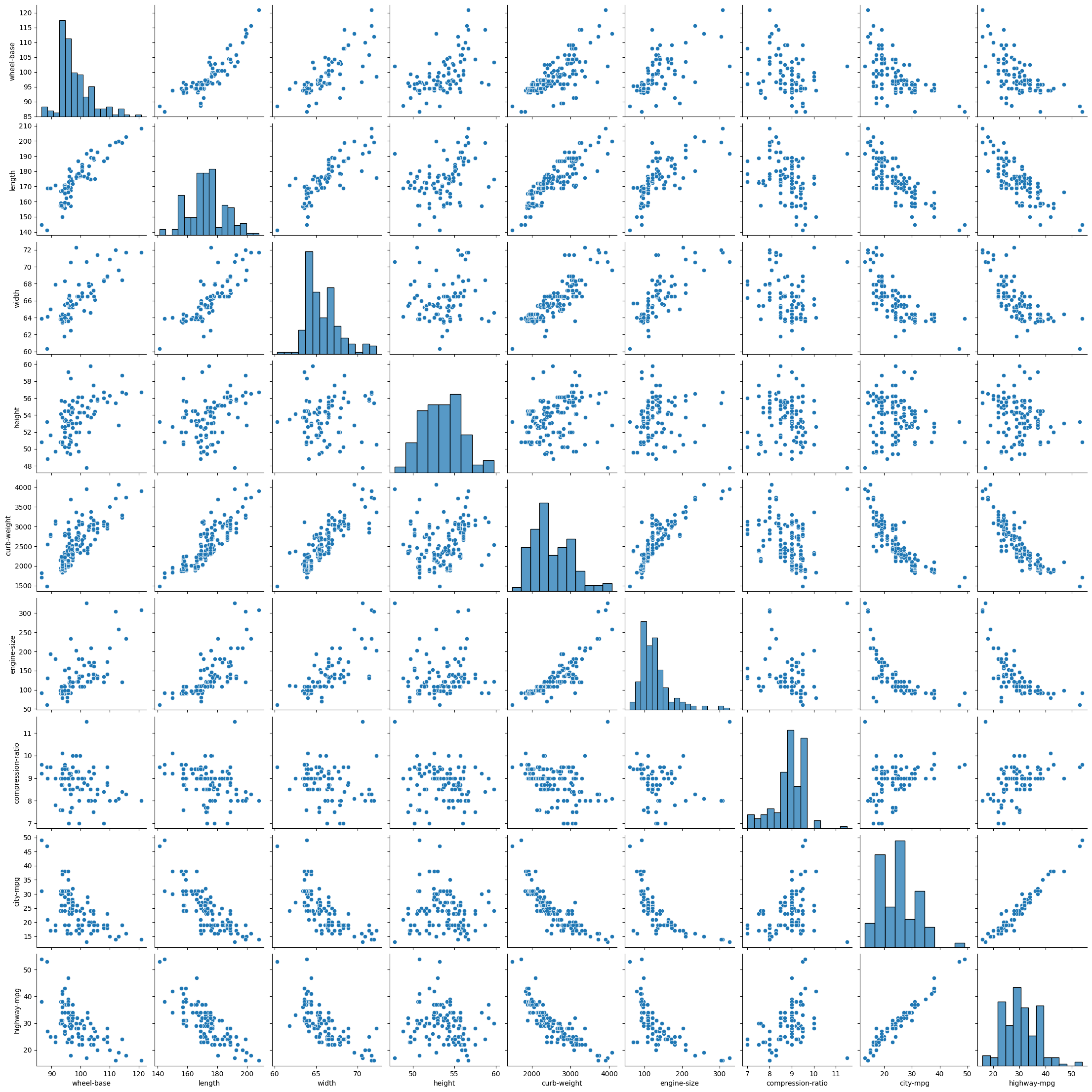
sns.pairplot(cars_df)
plt.show()

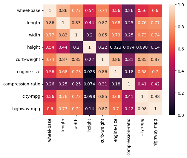
cars_corr = cars_df.corr(numeric_only=True)

sns.heatmap(np.abs(cars_corr), vmin = 0, vmax = 1, annot = True)
plt.show()

2.4.2. Modeling

Can we estimate fuel economy from other car specifications?

# Importing packages

from sklearn.linear_model import LinearRegression
from sklearn.preprocessing import StandardScaler
from sklearn.model_selection import train_test_split
from sklearn.datasets import make_regression
from sklearn.metrics import root_mean_squared_error, r2_score

# Chose features from correlation heatmap
# curb-weight most correlated, and height and compression independent of curb-weight
features = ['curb-weight', 'height', 'compression-ratio']
target = ['city-mpg']

X = cars_df[features]
y = cars_df[target]

In this case, we’ve selected the features ourselves, using intuition about correlation and avoiding colinearity between features. Our next steps:

1. Split the data into training (80%) and testing sets (20%). Each set includes both a features (X) and corresponding targets (y).

2. Normalize the data with StandardScalar. We do this because linear regression relies on a distance calculation.

   • First, create the StandardScalar transformer.

   • Fit the scaler to the feature vector of the training set. This calculates the mean and stdev for every feature.

   • Transform the training features using the scaler (X transformed to Z).

3. Create and fit the linear regression model.

   • Create the ‘template’ of a LinearRegression model.

   • Fit the model using the scaled features (Z) and targets (y) from the training set.

4. Make predictions.

   • Use the linear model to calculate the predicted targets (\(\hat y\)).

   • To make predictions using the test set, we must first scale the features.

5. Assess the model and visualize results.

   • Calculate RMSE and R²

   • Plot prediction vs actual

# Set aside data for testing
X_train, X_test, y_train, y_test = train_test_split(X, y, test_size = 0.2)

# Normalize the data

sc = StandardScaler()

# Calculates mean and stdev of X_train
sc.fit(X_train)

Z_train = sc.transform(X_train)

# Choose our model type (linear regression) and fit the parameters
linreg = LinearRegression()

# This fit is where we get values for thetas (our parameters)
linreg.fit(Z_train, y_train)

linreg.__dict__

{'fit_intercept': True,
 'copy_X': True,
 'tol': 1e-06,
 'n_jobs': None,
 'positive': False,
 'n_features_in_': 3,
 'coef_': array([[-5.2496175 ,  0.69410527,  0.96797346]]),
 'rank_': 3,
 'singular_': array([14.24305812, 11.83718112, 10.05069344]),
 'intercept_': array([24.72972973])}

2.4.3. Model Evaluation

# Make predictions with the model
y_pred_train = linreg.predict(Z_train)

# Make predictions on our test data

Z_test = sc.transform(X_test)
y_pred_test = linreg.predict(Z_test)

R2_train = r2_score(y_train, y_pred_train)
R2_test = r2_score(y_test, y_pred_test)

RMSE_train = root_mean_squared_error(y_train, y_pred_train)
RMSE_test = root_mean_squared_error(y_test, y_pred_test)

print(f'Train: \tR2: {R2_train:.3f}\tRMSE: {RMSE_train:.3f}')
print(f'Test: \tR2: {R2_test:.3f}\tRMSE: {RMSE_test:.3f}')

Train: 	R2: 0.746	RMSE: 3.227
Test: 	R2: 0.789	RMSE: 2.689

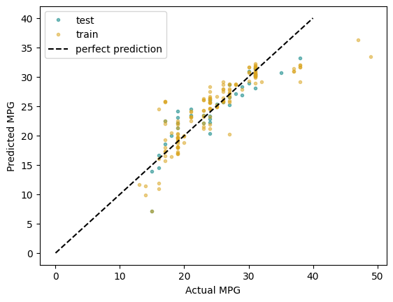
plt.plot(y_test, y_pred_test, '.', 
         color = 'teal', alpha = 0.5,
         label = 'test')
plt.plot(y_train, y_pred_train, '.', 
         color = 'goldenrod', alpha = 0.5,
         label = 'train')

plt.plot([0, 40], [0, 40], 'k--',
         label = 'perfect prediction')

plt.xlabel('Actual MPG')
plt.ylabel('Predicted MPG')
plt.legend()
plt.show()