
4.3. Example: King County Housing#
Can we do better fitting the King County Housing dataset with polynomial features?
import numpy as np
import matplotlib.pyplot as plt

import pandas as pd
from sklearn.model_selection import train_test_split
from sklearn.preprocessing import StandardScaler, PolynomialFeatures
from sklearn.linear_model import LassoCV
from sklearn.metrics import root_mean_squared_error, r2_score
4.3.1. Data cleaning#
housing_df = pd.read_csv('https://raw.githubusercontent.com/GettysburgDataScience/datasets/refs/heads/main/kc_house_data.csv')


# Change year built and year renovated to age of home and age of latest renovation
housing_df.loc[housing_df['yr_renovated']==0, 'yr_renovated'] = housing_df.loc[housing_df['yr_renovated']==0, 'yr_built']
housing_df['yr_sold'] = housing_df['date'].apply(lambda d: int(d[0:4]))
housing_df['age_built'] = housing_df['yr_sold'] - housing_df['yr_built']
housing_df['age_reno'] = housing_df['yr_sold'] - housing_df['yr_renovated']
# limit search to single-family homes (not apartments or apartment buildings)
housing_df = housing_df.query('3<=bedrooms<=5')
columns_to_drop = ['id','date', 'yr_built', 'yr_renovated', 'yr_sold', 'lat', 'long', 'waterfront', 'view', 'zipcode']
housing_df.drop(columns = columns_to_drop, inplace=True)

# Remove rows with missing data
housing_df.dropna(inplace=True)
housing_df.describe()
| price | bedrooms | bathrooms | sqft_living | sqft_lot | floors | condition | grade | sqft_above | sqft_basement | sqft_living15 | sqft_lot15 | age_built | age_reno | |
|---|---|---|---|---|---|---|---|---|---|---|---|---|---|---|
| count | 1.830700e+04 | 18307.000000 | 18307.000000 | 18307.000000 | 1.830700e+04 | 18307.000000 | 18307.000000 | 18307.000000 | 18307.000000 | 18307.000000 | 18307.000000 | 18307.00000 | 18307.000000 | 18307.000000 |
| mean | 5.578504e+05 | 3.550828 | 2.215191 | 2195.923090 | 1.548755e+04 | 1.523461 | 3.415087 | 7.784618 | 1887.189600 | 308.733490 | 2059.850931 | 13178.90490 | 40.502212 | 38.168078 |
| std | 3.689701e+05 | 0.649881 | 0.714074 | 870.622215 | 4.034957e+04 | 0.534261 | 0.646311 | 1.141706 | 811.950772 | 449.360359 | 684.036434 | 27242.83175 | 27.940249 | 27.194777 |
| min | 8.200000e+04 | 3.000000 | 0.500000 | 490.000000 | 5.200000e+02 | 1.000000 | 1.000000 | 4.000000 | 490.000000 | 0.000000 | 399.000000 | 651.00000 | -1.000000 | -1.000000 |
| 25% | 3.300000e+05 | 3.000000 | 1.750000 | 1570.000000 | 5.427500e+03 | 1.000000 | 3.000000 | 7.000000 | 1290.000000 | 0.000000 | 1550.000000 | 5440.00000 | 17.000000 | 15.000000 |
| 50% | 4.675000e+05 | 3.000000 | 2.250000 | 2030.000000 | 7.910000e+03 | 1.500000 | 3.000000 | 8.000000 | 1670.000000 | 0.000000 | 1920.000000 | 7875.00000 | 37.000000 | 35.000000 |
| 75% | 6.660000e+05 | 4.000000 | 2.500000 | 2640.000000 | 1.105200e+04 | 2.000000 | 4.000000 | 8.000000 | 2320.000000 | 600.000000 | 2440.000000 | 10350.00000 | 58.000000 | 55.000000 |
| max | 7.062500e+06 | 5.000000 | 6.750000 | 10040.000000 | 1.651359e+06 | 3.500000 | 5.000000 | 13.000000 | 8020.000000 | 4820.000000 | 6210.000000 | 871200.00000 | 115.000000 | 115.000000 |
4.3.2. Pre-processing#
target = 'price'

y = housing_df[target]
X = housing_df.drop(columns = target)
X.columns
Index(['bedrooms', 'bathrooms', 'sqft_living', 'sqft_lot', 'floors',
       'condition', 'grade', 'sqft_above', 'sqft_basement', 'sqft_living15',
       'sqft_lot15', 'age_built', 'age_reno'],
      dtype='object')
X_train, X_test, y_train, y_test = train_test_split(X, y, test_size = 0.2, random_state = 42)
poly = PolynomialFeatures(degree = 2, include_bias = False)
Xp_train = poly.fit_transform(X_train)
Xp_test = poly.transform(X_test)

sc = StandardScaler()
Z_train = sc.fit_transform(Xp_train)
Z_test = sc.transform(Xp_test)
# PolynomialFeatures returns a numpy array.
# Let's convert to a Pandas DataFrame for nicer viewing.
feature_names = poly.get_feature_names_out()

Xtrain_df = pd.DataFrame(data = Z_train, columns = feature_names)
Xtrain_df.head()
| bedrooms | bathrooms | sqft_living | sqft_lot | floors | condition | grade | sqft_above | sqft_basement | sqft_living15 | ... | sqft_living15^2 | sqft_living15 sqft_lot15 | sqft_living15 age_built | sqft_living15 age_reno | sqft_lot15^2 | sqft_lot15 age_built | sqft_lot15 age_reno | age_built^2 | age_built age_reno | age_reno^2 | |
|---|---|---|---|---|---|---|---|---|---|---|---|---|---|---|---|---|---|---|---|---|---|
| 0 | -0.849105 | -1.692939 | -0.741437 | -0.070810 | -0.984340 | 0.904126 | -0.686384 | -0.417690 | -0.683021 | -0.743171 | ... | -0.679743 | -0.232295 | 0.087422 | 0.180299 | -0.079117 | -0.014843 | 0.014964 | 0.130668 | 0.210905 | 0.223091 |
| 1 | 0.689326 | -1.692939 | -1.075351 | -0.281937 | -0.984340 | 0.904126 | -0.686384 | -0.776391 | -0.683021 | -1.051140 | ... | -0.859675 | -0.347587 | 1.111490 | 1.252352 | -0.084795 | -0.064999 | -0.039554 | 2.826634 | 3.076464 | 3.081207 |
| 2 | -0.849105 | 0.400012 | 0.847529 | 0.452976 | 0.896249 | -0.642711 | 1.067449 | 1.289229 | -0.683021 | 2.439168 | ... | 2.710742 | 1.397592 | -0.463746 | -0.396695 | 0.026973 | 0.007628 | 0.039389 | -0.772480 | -0.749057 | -0.734378 |
| 3 | 0.689326 | 0.400012 | 0.055349 | 0.538262 | 0.896249 | -0.642711 | 0.190533 | 0.438243 | -0.683021 | 0.271658 | ... | 0.098232 | -0.014652 | -0.637546 | -0.578639 | -0.070591 | -0.235036 | -0.224381 | -0.715450 | -0.688440 | -0.673918 |
| 4 | -0.849105 | 0.400012 | -0.453581 | -0.285550 | 0.896249 | -0.642711 | 0.190533 | -0.108466 | -0.683021 | -0.376542 | ... | -0.431443 | -0.307025 | -0.560526 | -0.498010 | -0.084333 | -0.362655 | -0.363101 | -0.606575 | -0.572715 | -0.558494 |
5 rows × 104 columns
4.3.2.1. Fitting the model#
test_alphas = np.logspace(-2,4, 19)
lasso = LassoCV(alphas=test_alphas, cv=5, max_iter = 30000)
lasso.fit(Z_train, y_train)
LassoCV(alphas=array([1.00000000e-02, 2.15443469e-02, 4.64158883e-02, 1.00000000e-01,
       2.15443469e-01, 4.64158883e-01, 1.00000000e+00, 2.15443469e+00,
       4.64158883e+00, 1.00000000e+01, 2.15443469e+01, 4.64158883e+01,
       1.00000000e+02, 2.15443469e+02, 4.64158883e+02, 1.00000000e+03,
       2.15443469e+03, 4.64158883e+03, 1.00000000e+04]),
        cv=5, max_iter=30000)
In a Jupyter environment, please rerun this cell to show the HTML representation or trust the notebook. On GitHub, the HTML representation is unable to render, please try loading this page with nbviewer.org.
Parameters
| eps | 0.001 | |
| n_alphas | 'deprecated' | |
| alphas | array([1.0000...00000000e+04]) | |
| fit_intercept | True | |
| precompute | 'auto' | |
| max_iter | 30000 | |
| tol | 0.0001 | |
| copy_X | True | |
| cv | 5 | |
| verbose | False | |
| n_jobs | None | |
| positive | False | |
| random_state | None | |
| selection | 'cyclic' |
Let’s inspect the fit coefficients.
print(f'The best alpha = {lasso.alpha_:.5g}')

for k, (feature, weight) in enumerate(zip(feature_names, lasso.coef_)):
    print(f'{k:>3}.\t{feature:>20} \t {weight:+0.4f}')
The best alpha = 464.16
  0.	            bedrooms 	 -0.0000
  1.	           bathrooms 	 -0.0000
  2.	         sqft_living 	 -101376.0206
  3.	            sqft_lot 	 +46021.0372
  4.	              floors 	 +0.0000
  5.	           condition 	 -27133.7048
  6.	               grade 	 -5523.0165
  7.	          sqft_above 	 -0.0000
  8.	       sqft_basement 	 -0.0000
  9.	       sqft_living15 	 -94884.1463
 10.	          sqft_lot15 	 +17692.5381
 11.	           age_built 	 -46645.1272
 12.	            age_reno 	 -0.0000
 13.	          bedrooms^2 	 -0.0000
 14.	  bedrooms bathrooms 	 -0.0000
 15.	bedrooms sqft_living 	 -0.0000
 16.	   bedrooms sqft_lot 	 +0.0000
 17.	     bedrooms floors 	 +0.0000
 18.	  bedrooms condition 	 -0.0000
 19.	      bedrooms grade 	 -0.0000
 20.	 bedrooms sqft_above 	 +0.0000
 21.	bedrooms sqft_basement 	 -41073.5220
 22.	bedrooms sqft_living15 	 -5174.5315
 23.	 bedrooms sqft_lot15 	 +0.0000
 24.	  bedrooms age_built 	 +0.0000
 25.	   bedrooms age_reno 	 +0.0000
 26.	         bathrooms^2 	 +0.0000
 27.	bathrooms sqft_living 	 +26984.2715
 28.	  bathrooms sqft_lot 	 -0.0000
 29.	    bathrooms floors 	 +0.0000
 30.	 bathrooms condition 	 -0.0000
 31.	     bathrooms grade 	 +14123.4192
 32.	bathrooms sqft_above 	 +64996.6286
 33.	bathrooms sqft_basement 	 +0.0000
 34.	bathrooms sqft_living15 	 +0.0000
 35.	bathrooms sqft_lot15 	 -18833.5261
 36.	 bathrooms age_built 	 -26288.6649
 37.	  bathrooms age_reno 	 -0.0000
 38.	       sqft_living^2 	 +0.0000
 39.	sqft_living sqft_lot 	 -56149.1012
 40.	  sqft_living floors 	 +0.0000
 41.	sqft_living condition 	 +0.0000
 42.	   sqft_living grade 	 +83109.9795
 43.	sqft_living sqft_above 	 +111425.8364
 44.	sqft_living sqft_basement 	 +0.0000
 45.	sqft_living sqft_living15 	 +0.0000
 46.	sqft_living sqft_lot15 	 -26413.6870
 47.	sqft_living age_built 	 +18003.4714
 48.	sqft_living age_reno 	 -41533.4816
 49.	          sqft_lot^2 	 +4283.5250
 50.	     sqft_lot floors 	 +10090.2621
 51.	  sqft_lot condition 	 +0.0000
 52.	      sqft_lot grade 	 +0.0000
 53.	 sqft_lot sqft_above 	 -0.0000
 54.	sqft_lot sqft_basement 	 -0.0000
 55.	sqft_lot sqft_living15 	 +0.0000
 56.	 sqft_lot sqft_lot15 	 +13441.8684
 57.	  sqft_lot age_built 	 -19708.9748
 58.	   sqft_lot age_reno 	 -4501.0125
 59.	            floors^2 	 +31406.9616
 60.	    floors condition 	 +28889.9229
 61.	        floors grade 	 +0.0000
 62.	   floors sqft_above 	 +0.0000
 63.	floors sqft_basement 	 +0.0000
 64.	floors sqft_living15 	 -67310.6046
 65.	   floors sqft_lot15 	 -0.0000
 66.	    floors age_built 	 -40429.2672
 67.	     floors age_reno 	 -0.0000
 68.	         condition^2 	 -0.0000
 69.	     condition grade 	 -0.0000
 70.	condition sqft_above 	 -0.0000
 71.	condition sqft_basement 	 +2897.2754
 72.	condition sqft_living15 	 +70731.1051
 73.	condition sqft_lot15 	 +0.0000
 74.	 condition age_built 	 +0.0000
 75.	  condition age_reno 	 +0.0000
 76.	             grade^2 	 +115811.0922
 77.	    grade sqft_above 	 +0.0000
 78.	 grade sqft_basement 	 +57579.8073
 79.	 grade sqft_living15 	 -0.0000
 80.	    grade sqft_lot15 	 -0.0000
 81.	     grade age_built 	 -0.0000
 82.	      grade age_reno 	 -0.0000
 83.	        sqft_above^2 	 +0.0000
 84.	sqft_above sqft_basement 	 +55471.8912
 85.	sqft_above sqft_living15 	 -0.0000
 86.	sqft_above sqft_lot15 	 -0.0000
 87.	sqft_above age_built 	 +12878.1279
 88.	 sqft_above age_reno 	 -6179.9539
 89.	     sqft_basement^2 	 -7067.8496
 90.	sqft_basement sqft_living15 	 +6867.9534
 91.	sqft_basement sqft_lot15 	 -10045.4611
 92.	sqft_basement age_built 	 +0.0000
 93.	sqft_basement age_reno 	 -0.0000
 94.	     sqft_living15^2 	 +36210.6433
 95.	sqft_living15 sqft_lot15 	 +0.0000
 96.	sqft_living15 age_built 	 +207428.9831
 97.	sqft_living15 age_reno 	 -29787.7428
 98.	        sqft_lot15^2 	 +19697.3695
 99.	sqft_lot15 age_built 	 -3161.6480
100.	 sqft_lot15 age_reno 	 -7938.2271
101.	         age_built^2 	 -0.0000
102.	  age_built age_reno 	 +0.0000
103.	          age_reno^2 	 +56995.4397
Same as above, but now the coefficients are in order of importance.
# Same as above but sorted by importance

# np.argsort returns the order of indices in the reordered array
# I'm sorting the absolute value of the coefficients because it's the size of the coeff that's important

sort_order = np.argsort(np.abs(lasso.coef_))[::-1]

for k, (feature, weight) in enumerate(zip(feature_names[sort_order], lasso.coef_[sort_order]), start = 1):
    print(f'{k:>3}.\t{feature:>40} \t {weight:+0.4f}')
  1.	                 sqft_living15 age_built 	 +207428.9831
  2.	                                 grade^2 	 +115811.0922
  3.	                  sqft_living sqft_above 	 +111425.8364
  4.	                             sqft_living 	 -101376.0206
  5.	                           sqft_living15 	 -94884.1463
  6.	                       sqft_living grade 	 +83109.9795
  7.	                 condition sqft_living15 	 +70731.1051
  8.	                    floors sqft_living15 	 -67310.6046
  9.	                    bathrooms sqft_above 	 +64996.6286
 10.	                     grade sqft_basement 	 +57579.8073
 11.	                              age_reno^2 	 +56995.4397
 12.	                    sqft_living sqft_lot 	 -56149.1012
 13.	                sqft_above sqft_basement 	 +55471.8912
 14.	                               age_built 	 -46645.1272
 15.	                                sqft_lot 	 +46021.0372
 16.	                    sqft_living age_reno 	 -41533.4816
 17.	                  bedrooms sqft_basement 	 -41073.5220
 18.	                        floors age_built 	 -40429.2672
 19.	                         sqft_living15^2 	 +36210.6433
 20.	                                floors^2 	 +31406.9616
 21.	                  sqft_living15 age_reno 	 -29787.7428
 22.	                        floors condition 	 +28889.9229
 23.	                               condition 	 -27133.7048
 24.	                   bathrooms sqft_living 	 +26984.2715
 25.	                  sqft_living sqft_lot15 	 -26413.6870
 26.	                     bathrooms age_built 	 -26288.6649
 27.	                      sqft_lot age_built 	 -19708.9748
 28.	                            sqft_lot15^2 	 +19697.3695
 29.	                    bathrooms sqft_lot15 	 -18833.5261
 30.	                   sqft_living age_built 	 +18003.4714
 31.	                              sqft_lot15 	 +17692.5381
 32.	                         bathrooms grade 	 +14123.4192
 33.	                     sqft_lot sqft_lot15 	 +13441.8684
 34.	                    sqft_above age_built 	 +12878.1279
 35.	                         sqft_lot floors 	 +10090.2621
 36.	                sqft_basement sqft_lot15 	 -10045.4611
 37.	                     sqft_lot15 age_reno 	 -7938.2271
 38.	                         sqft_basement^2 	 -7067.8496
 39.	             sqft_basement sqft_living15 	 +6867.9534
 40.	                     sqft_above age_reno 	 -6179.9539
 41.	                                   grade 	 -5523.0165
 42.	                  bedrooms sqft_living15 	 -5174.5315
 43.	                       sqft_lot age_reno 	 -4501.0125
 44.	                              sqft_lot^2 	 +4283.5250
 45.	                    sqft_lot15 age_built 	 -3161.6480
 46.	                 condition sqft_basement 	 +2897.2754
 47.	                        bathrooms floors 	 +0.0000
 48.	                     bathrooms condition 	 -0.0000
 49.	                                  floors 	 +0.0000
 50.	                               bathrooms 	 -0.0000
 51.	                 bathrooms sqft_basement 	 +0.0000
 52.	                 bathrooms sqft_living15 	 +0.0000
 53.	                                age_reno 	 -0.0000
 54.	                      bathrooms sqft_lot 	 -0.0000
 55.	                             bathrooms^2 	 +0.0000
 56.	                       bedrooms age_reno 	 +0.0000
 57.	                      bedrooms age_built 	 +0.0000
 58.	                     bedrooms sqft_lot15 	 +0.0000
 59.	                     bedrooms sqft_above 	 +0.0000
 60.	                              sqft_above 	 -0.0000
 61.	                          bedrooms grade 	 -0.0000
 62.	                      bedrooms condition 	 -0.0000
 63.	                       bedrooms sqft_lot 	 +0.0000
 64.	                           sqft_basement 	 -0.0000
 65.	                    bedrooms sqft_living 	 -0.0000
 66.	                      bedrooms bathrooms 	 -0.0000
 67.	                              bedrooms^2 	 -0.0000
 68.	                         bedrooms floors 	 +0.0000
 69.	                      sqft_lot condition 	 +0.0000
 70.	                      bathrooms age_reno 	 -0.0000
 71.	                          grade age_reno 	 -0.0000
 72.	                     condition age_built 	 +0.0000
 73.	                      condition age_reno 	 +0.0000
 74.	                        grade sqft_above 	 +0.0000
 75.	                     grade sqft_living15 	 -0.0000
 76.	                        grade sqft_lot15 	 -0.0000
 77.	                         grade age_built 	 -0.0000
 78.	                            sqft_above^2 	 +0.0000
 79.	                    condition sqft_above 	 -0.0000
 80.	                sqft_above sqft_living15 	 -0.0000
 81.	                   sqft_above sqft_lot15 	 -0.0000
 82.	                 sqft_basement age_built 	 +0.0000
 83.	                  sqft_basement age_reno 	 -0.0000
 84.	                sqft_living15 sqft_lot15 	 +0.0000
 85.	                             age_built^2 	 -0.0000
 86.	                    condition sqft_lot15 	 +0.0000
 87.	                         condition grade 	 -0.0000
 88.	                           sqft_living^2 	 +0.0000
 89.	                     sqft_lot sqft_above 	 -0.0000
 90.	                      sqft_living floors 	 +0.0000
 91.	                   sqft_living condition 	 +0.0000
 92.	               sqft_living sqft_basement 	 +0.0000
 93.	               sqft_living sqft_living15 	 +0.0000
 94.	                      age_built age_reno 	 +0.0000
 95.	                          sqft_lot grade 	 +0.0000
 96.	                  sqft_lot sqft_basement 	 -0.0000
 97.	                             condition^2 	 -0.0000
 98.	                  sqft_lot sqft_living15 	 +0.0000
 99.	                            floors grade 	 +0.0000
100.	                       floors sqft_above 	 +0.0000
101.	                    floors sqft_basement 	 +0.0000
102.	                       floors sqft_lot15 	 -0.0000
103.	                         floors age_reno 	 -0.0000
104.	                                bedrooms 	 -0.0000
# Assessing model
y_lasso_test = lasso.predict(Z_test)
y_lasso_train = lasso.predict(Z_train)


rmse_lasso_train = root_mean_squared_error(y_train, y_lasso_train)
r2_lasso_train = r2_score(y_train, y_lasso_train)

rmse_lasso_test = root_mean_squared_error(y_test, y_lasso_test)
r2_lasso_test = r2_score(y_test, y_lasso_test)

print("Lasso Regression Performance (Standardized Target):\n")
print(f"  Train RMSE: {rmse_lasso_train:.3f}")
print(f"  Test  RMSE: {rmse_lasso_test:.3f}\n")

print(f"  Train R^2: {r2_lasso_train:.3f}")
print(f"  Test  R^2: {r2_lasso_test:.3f}")
Lasso Regression Performance (Standardized Target):

  Train RMSE: 199672.389
  Test  RMSE: 205729.638

  Train R^2: 0.709
  Test  R^2: 0.683
plt.plot(y_train, y_lasso_train, '.', color = 'firebrick', label = 'train', alpha = 0.2)
plt.plot(y_test, y_lasso_test, '.', color = 'teal', label = 'test', alpha = 0.2)

plimits = [0, 7000000]
plt.plot(plimits, plimits, '--', color = 'goldenrod')

plt.xlabel('Actual Sale Price ($)')
plt.ylabel('Predicted Sale Price ($)')
plt.show()
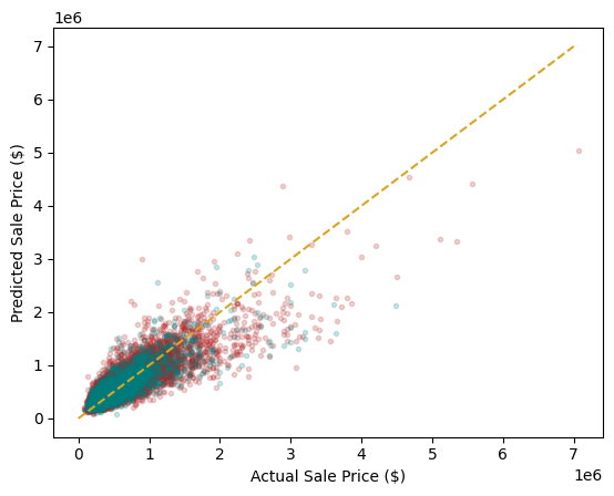
Question
Inspecting this result, where is the model over- or under-estimating house value? Can you think of a fix for this problem?