8. PCA: Examples and Observations

Principle Component Analysis (PCA) is one of the more complex concepts in data science. In this notebook, we look at some examples and make some general observations as to the (beneficial) effects and uses of PCA.

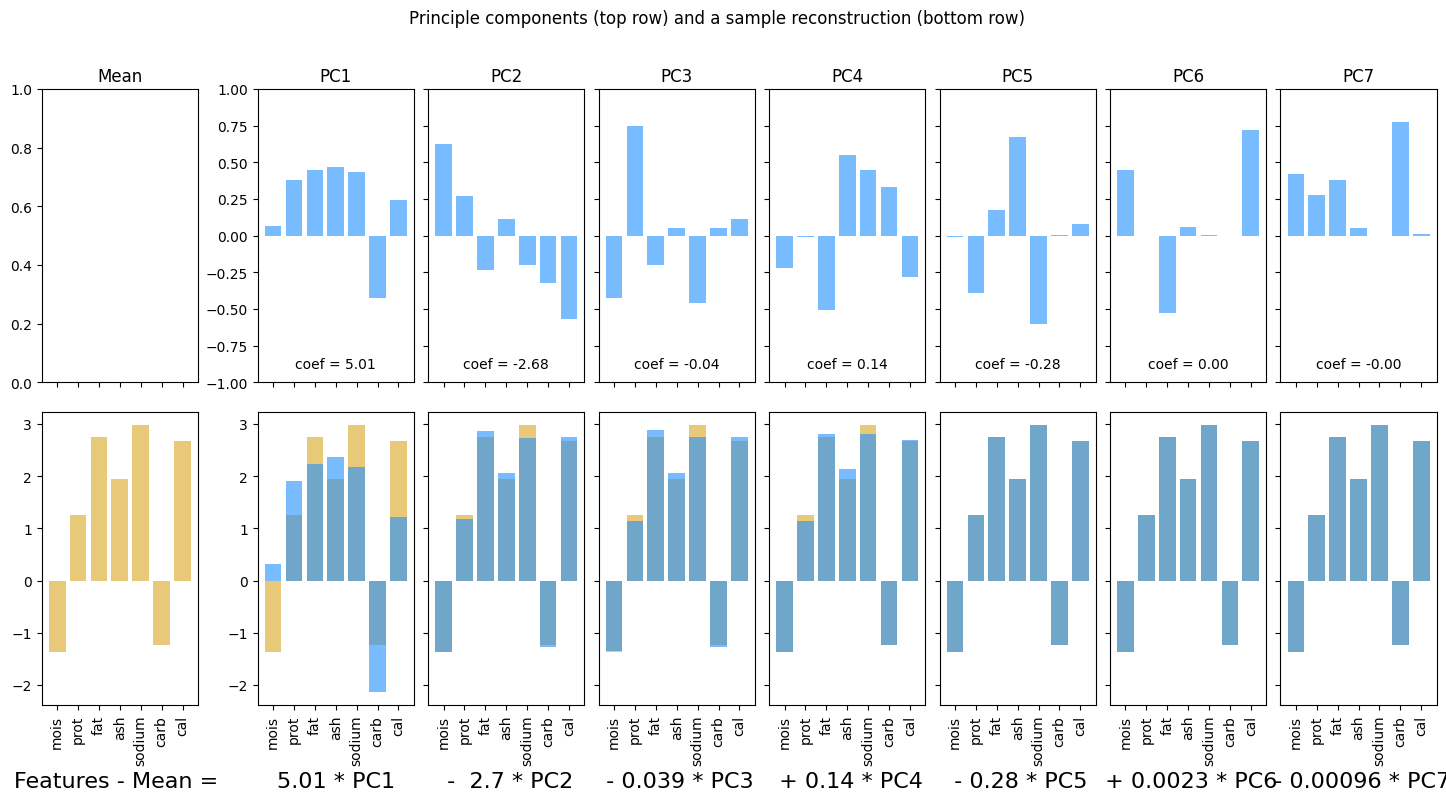
Working through the examples, observe:

• Features that vary together appear in the same Principle Components. As a result, PCA solves the co-linearity problem.

• You can approximately reconstruct the original feature values with fewer than all the PCs.

import numpy as np
import pandas as pd

import matplotlib.pyplot as plt

from sklearn.decomposition import PCA
from sklearn.preprocessing import StandardScaler

Show code cell source Hide code cell source

def plotPCA(data, pca=None, num_components = None, idx = 0, feature_names = None):

# plot PCA components and a reconstruction of one data instance

    if pca is None:
        if num_components is None:
            pca = PCA()
        else:
            pca = PCA(n_components = num_components)
    
    X = pca.fit_transform(data)

    if num_components is None:
        num_components = pca.n_components_
    
    
    if isinstance(data, pd.DataFrame):
        x0 = data.iloc[idx,:]
    else:
        x0 = data[idx,:]
        
    x_pca = np.zeros_like(x0)
    
    coeffs = X[idx,:]
    
    if feature_names is None:
        try:
            feature_names = pca.feature_names_in_
        except:
            feature_names = [str(i) for i in range(data.shape[1])]

    C0 = 'goldenrod'
    C1 = 'dodgerblue'
    alpha = 0.6
    

    offset = 2
    num_cols = num_components + offset
    width_ratios = [1, 0.2] + [1]*num_components
        
    fig, ax = plt.subplots(2, num_cols, figsize = ((num_cols)*2, 8), 
                        sharex = True, sharey = False,
                        gridspec_kw = dict(width_ratios=width_ratios,
                                            hspace = 0.1, wspace = 0.1)                       
                        )
    
    if not np.all(np.isclose(pca.mean_, 0)):
        ax[0, 0].bar(feature_names, pca.mean_, color = C1, alpha = alpha)
        ax[0, 0].bar(feature_names, x0, color = C0, alpha = alpha)
        
        ax[0, 0].sharey(ax[1,offset])
    
    ax[0,0].set_title('Mean')

    ax[1, 0].bar(feature_names, x0-pca.mean_, color = C0, alpha = alpha)
    ax[1, 0].bar(feature_names, x_pca, color = C1, alpha = alpha)
    ax[1, 0].set_xlabel('Features - Mean = ', fontsize = 16)
    ax[1, 0].tick_params(axis='x', labelrotation = 90, )
    ax[1, 0].sharey(ax[1,offset])


    # ax[0, 2].set_title(f'PC1')   

    ax[0,1].set_visible(False)
    ax[1,1].set_visible(False)

    for r_idx, (r, coef) in enumerate(zip(pca.components_, coeffs)):
        x_pca += coef * r
        ax[0, r_idx+offset].bar(feature_names, r, color = C1, alpha = alpha)
        ax[0, r_idx+offset].text(0.5, 0.05, f'coef = {coef:0.2f}', ha = 'center', transform=ax[0, r_idx+offset].transAxes)
        
        ax[1, r_idx+offset].bar(feature_names, x0-pca.mean_, color = C0, alpha = alpha)
        ax[1, r_idx+offset].bar(feature_names, x_pca, alpha = alpha, color = C1)
        
        if r_idx == 0:
            ax_str = f'{coef:0.2f} * PC1'
        
        if r_idx>0:
            ax[0, r_idx+offset].sharey(ax[0,offset])
            ax[1, r_idx+offset].sharey(ax[1,offset])
            plt.setp(ax[0,r_idx+offset].get_yticklabels(), visible=False)
            plt.setp(ax[1,r_idx+offset].get_yticklabels(), visible=False)
            
            if coef > 0:
                ax_str = f' + {coef:4.2} * PC{r_idx+1}'
            elif coef < 0:
                ax_str = f' - {-1*coef:4.2} * PC{r_idx+1}'
            else:
                ax_str = f' + 0'
                        
        ax[0, r_idx+offset].set_title(f'PC{r_idx+1}')   
        ax[1, r_idx+offset].set_xlabel(ax_str, fontsize = 16)
        ax[1, r_idx+offset].tick_params(axis='x', labelrotation = 90, )


    ax[0,2].set_ylim([-1, 1])
    fig.suptitle('Principle components (top row) and a sample reconstruction (bottom row)')

    return pca, fig, ax

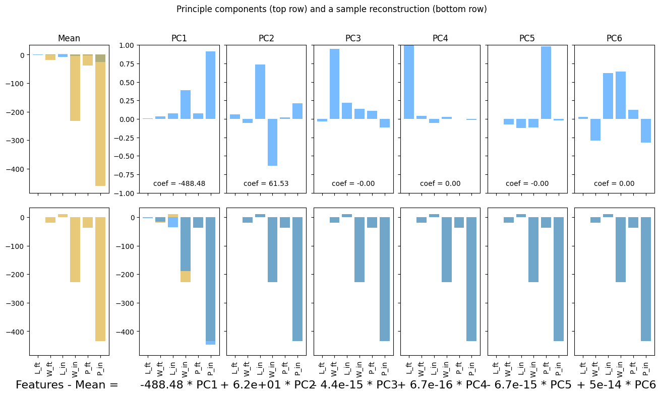
8.1. Example 0: Synthetic data (boxes)

num_data = 100

boxes_dict = {'L_ft': 5*np.random.randn(num_data),
              'W_ft': 10*np.random.randn(num_data)
              }

boxes_df = pd.DataFrame(boxes_dict)
boxes_df

	L_ft	W_ft
0	-3.799786	1.491786
1	6.050738	-4.238306
2	-11.037197	6.851790
3	6.792352	-4.045675
4	-6.838963	-5.197603
...	...	...
95	2.344248	-11.745888
96	-3.561784	-0.456870
97	-2.896416	8.947900
98	-1.264895	18.349202
99	2.268445	1.091549

100 rows × 2 columns

boxes_df[['L_in', 'W_in']] = boxes_df[['L_ft','W_ft']]*12
boxes_df['P_ft'] = 2*(boxes_df['L_ft']+boxes_df['W_ft'])
boxes_df['P_in'] = 2*(boxes_df['L_in']+boxes_df['W_in'])

boxes_df

	L_ft	W_ft	L_in	W_in	P_ft	P_in
0	-3.799786	1.491786	-45.597430	17.901432	-4.616000	-55.391995
1	6.050738	-4.238306	72.608856	-50.859672	3.624864	43.498368
2	-11.037197	6.851790	-132.446362	82.221484	-8.370813	-100.449757
3	6.792352	-4.045675	81.508220	-48.548094	5.493354	65.920251
4	-6.838963	-5.197603	-82.067555	-62.371241	-24.073133	-288.877592
...	...	...	...	...	...	...
95	2.344248	-11.745888	28.130974	-140.950657	-18.803280	-225.639366
96	-3.561784	-0.456870	-42.741409	-5.482442	-8.037308	-96.447701
97	-2.896416	8.947900	-34.756995	107.374806	12.102968	145.235621
98	-1.264895	18.349202	-15.178746	220.190428	34.168614	410.023365
99	2.268445	1.091549	27.221338	13.098589	6.719988	80.639853

100 rows × 6 columns

pca, fig, ax = plotPCA(boxes_df)
plt.show()

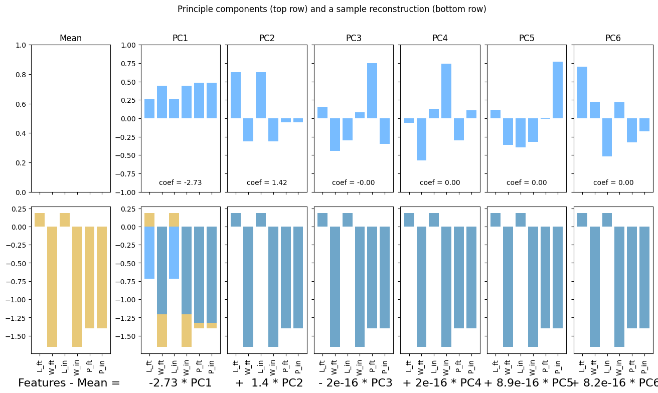
ss = StandardScaler()
boxes_scaled = ss.fit_transform(boxes_df)
boxes_scaled_df = pd.DataFrame(boxes_scaled, columns = boxes_df.columns)

pca_scaled, fig, ax = plotPCA(boxes_scaled_df)
plt.show()

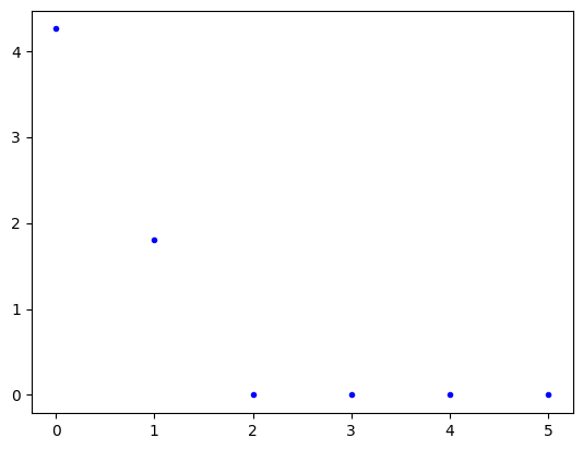
plt.plot(pca_scaled.explained_variance_, 'b.')
plt.show()

8.2. Example 1: Macro-nutrients

macros_df = pd.read_csv('https://raw.githubusercontent.com/f-imp/Principal-Component-Analysis-PCA-over-3-datasets/refs/heads/master/datasets/Pizza.csv')
macros_df.head()

	brand	id	mois	prot	fat	ash	sodium	carb	cal
0	A	14069	27.82	21.43	44.87	5.11	1.77	0.77	4.93
1	A	14053	28.49	21.26	43.89	5.34	1.79	1.02	4.84
2	A	14025	28.35	19.99	45.78	5.08	1.63	0.80	4.95
3	A	14016	30.55	20.15	43.13	4.79	1.61	1.38	4.74
4	A	14005	30.49	21.28	41.65	4.82	1.64	1.76	4.67

features_to_keep = ['mois', 'prot', 'fat', 'ash', 'sodium', 'carb', 'cal']

macros_df = macros_df[features_to_keep]
macros_df

	mois	prot	fat	ash	sodium	carb	cal
0	27.82	21.43	44.87	5.11	1.77	0.77	4.93
1	28.49	21.26	43.89	5.34	1.79	1.02	4.84
2	28.35	19.99	45.78	5.08	1.63	0.80	4.95
3	30.55	20.15	43.13	4.79	1.61	1.38	4.74
4	30.49	21.28	41.65	4.82	1.64	1.76	4.67
...	...	...	...	...	...	...	...
295	44.91	11.07	17.00	2.49	0.66	25.36	2.91
296	43.15	11.79	18.46	2.43	0.67	24.17	3.10
297	44.55	11.01	16.03	2.43	0.64	25.98	2.92
298	47.60	10.43	15.18	2.32	0.56	24.47	2.76
299	46.84	9.91	15.50	2.27	0.57	25.48	2.81

300 rows × 7 columns

pca = PCA(n_components = 6)
macros_pca = pca.fit_transform(macros_df)

pca_df = pd.DataFrame(data = pca.components_, columns = macros_df.columns)
pca_df

/Users/eatai/.pyenv/versions/3.13.1/envs/datascience/lib/python3.13/site-packages/sklearn/decomposition/_base.py:148: RuntimeWarning: divide by zero encountered in matmul
  X_transformed = X @ self.components_.T
/Users/eatai/.pyenv/versions/3.13.1/envs/datascience/lib/python3.13/site-packages/sklearn/decomposition/_base.py:148: RuntimeWarning: overflow encountered in matmul
  X_transformed = X @ self.components_.T
/Users/eatai/.pyenv/versions/3.13.1/envs/datascience/lib/python3.13/site-packages/sklearn/decomposition/_base.py:148: RuntimeWarning: invalid value encountered in matmul
  X_transformed = X @ self.components_.T

	mois	prot	fat	ash	sodium	carb	cal
0	-0.276963	-0.266941	-0.278934	-0.055434	-0.011142	0.878084	-0.000603
1	0.747074	-0.055733	-0.657845	-0.040604	-0.023814	0.006818	-0.061254
2	-0.352016	0.809718	-0.467976	0.022225	-0.026245	-0.012469	-0.010062
3	-0.195900	-0.255747	-0.259802	0.871443	0.201453	-0.164525	-0.040678
4	0.059475	0.083719	0.035776	-0.166634	0.978316	0.057470	0.001497
5	0.440974	0.443490	0.448624	0.450220	-0.030463	0.444405	-0.080452

feature_names = list(macros_df.columns)
ss = StandardScaler()

X = ss.fit_transform(macros_df)
fig, ax = plotPCA(X, feature_names = feature_names)

/Users/eatai/.pyenv/versions/3.13.1/envs/datascience/lib/python3.13/site-packages/sklearn/decomposition/_base.py:148: RuntimeWarning: divide by zero encountered in matmul
  X_transformed = X @ self.components_.T
/Users/eatai/.pyenv/versions/3.13.1/envs/datascience/lib/python3.13/site-packages/sklearn/decomposition/_base.py:148: RuntimeWarning: overflow encountered in matmul
  X_transformed = X @ self.components_.T
/Users/eatai/.pyenv/versions/3.13.1/envs/datascience/lib/python3.13/site-packages/sklearn/decomposition/_base.py:148: RuntimeWarning: invalid value encountered in matmul
  X_transformed = X @ self.components_.T

---------------------------------------------------------------------------
ValueError                                Traceback (most recent call last)
Cell In[11], line 5
      2 ss = StandardScaler()
      4 X = ss.fit_transform(macros_df)
----> 5 fig, ax = plotPCA(X, feature_names = feature_names)

ValueError: too many values to unpack (expected 2)

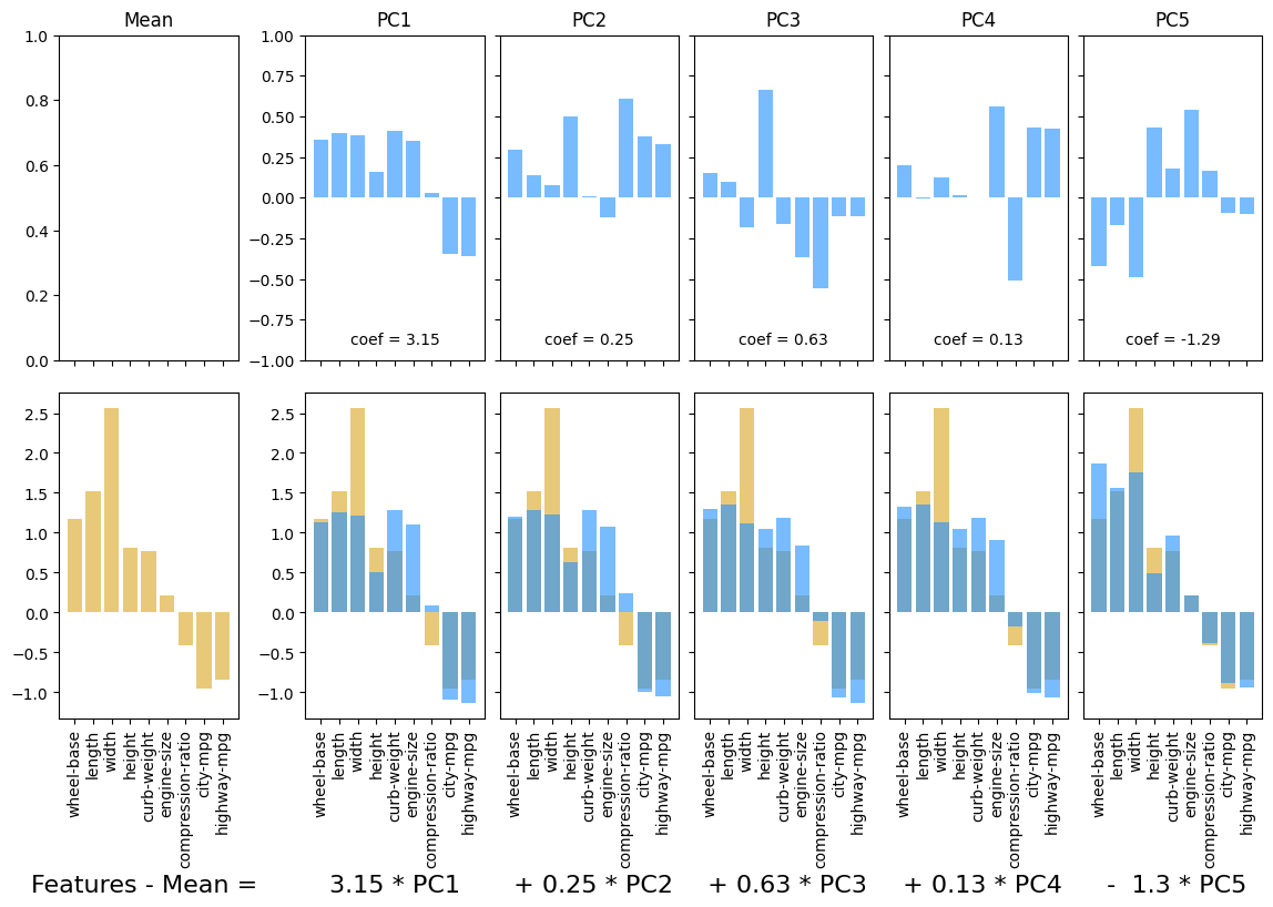
8.3. Example 2: Automobile specs

cars_df = pd.read_csv('https://raw.githubusercontent.com/shreyamdg/automobile-data-set-analysis/refs/heads/master/cars.csv')
cars_df.head()

	Unnamed: 0	symboling	normalized-losses	make	fuel-type	aspiration	num-of-doors	body-style	drive-wheels	engine-location	...	engine-size	fuel-system	bore	stroke	compression-ratio	horsepower	peak-rpm	city-mpg	highway-mpg	price
0	0	3	?	alfa-romero	gas	std	two	convertible	rwd	front	...	130	mpfi	3.47	2.68	9.0	111	5000	21	27	13495
1	1	3	?	alfa-romero	gas	std	two	convertible	rwd	front	...	130	mpfi	3.47	2.68	9.0	111	5000	21	27	16500
2	2	1	?	alfa-romero	gas	std	two	hatchback	rwd	front	...	152	mpfi	2.68	3.47	9.0	154	5000	19	26	16500
3	3	2	164	audi	gas	std	four	sedan	fwd	front	...	109	mpfi	3.19	3.40	10.0	102	5500	24	30	13950
4	4	2	164	audi	gas	std	four	sedan	4wd	front	...	136	mpfi	3.19	3.40	8.0	115	5500	18	22	17450

5 rows × 27 columns

specs_df = cars_df.select_dtypes(include = 'number').drop(columns = ['Unnamed: 0', 'symboling'])
names_df = cars_df[['make',  'num-of-doors', 'body-style', 'fuel-type']]

idx = 7

ss = StandardScaler()
X = ss.fit_transform(specs_df)
feature_names = list(specs_df.columns)

display(names_df.iloc[[7]])

plotPCA(X, num_components = 5, feature_names = feature_names, idx = idx)
plt.show()

	make	num-of-doors	body-style	fuel-type
7	audi	four	wagon	gas